Excel’s checkbox tool helps you to manage your numbers, track task progress, and display data more clearly. One of Excel’s less-known gems is its ability to produce a timestamp when a checkbox is checked. Here’s how you can make this happen.
Step 1: Format Your Table
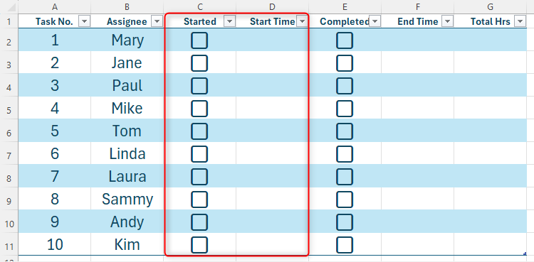
In my case, I have a list of individuals due to complete a task, and I’m going to use timestamped checkboxes to track when they started the task, when they finished it, and how long it took them to complete it.
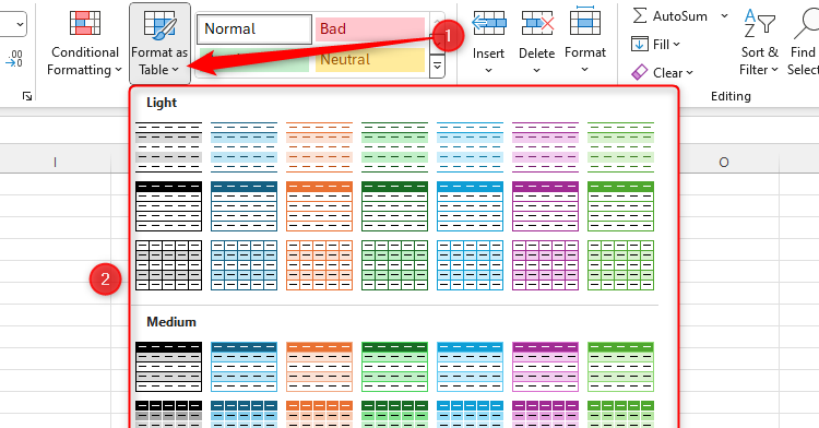
After naming your columns in row 1, the next stage is to format your table so that it’s a little easier on the eye, and any calculations will duplicate automatically. To do this, select any cell that contains data, click “Format As Table” in the Home tab, and choose a design that works for you.
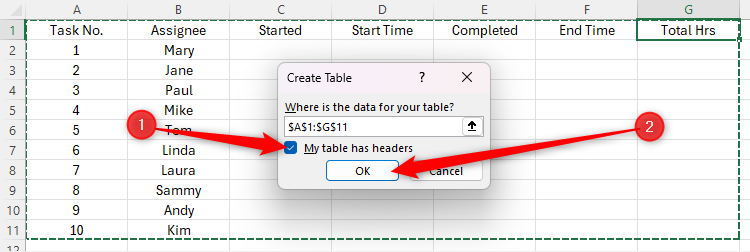
Since you have already named your columns, check “My Table Has Headers” when the Create Table dialog box appears, and click “OK.”
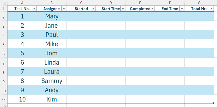
The table is now ready for you to move to the next step.
Step 2: Set Your Time Data Type
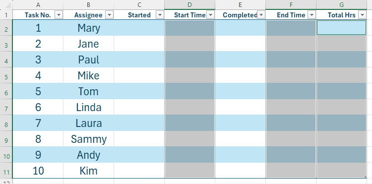
Before you add any calculations or checkboxes, you need to tell Excel that certain columns (in my case, columns D, F, and G) will output a time by changing the data type for these cells.
If you have only one column requiring a time output, simply select all the data cells in that column in your table. If you have more than one column that will display a time, hold Ctrl while you select them individually.
If your table contains hundreds of rows, selecting the cells manually could take a long time! In this case, select the first data cell in a relevant column, and press Ctrl+Shift+Down. Then, hold Ctrl, and select the first data cell in the next relevant column, and press Ctrl+Shift+Down. Repeat this process until all relevant columns’ cells are selected.
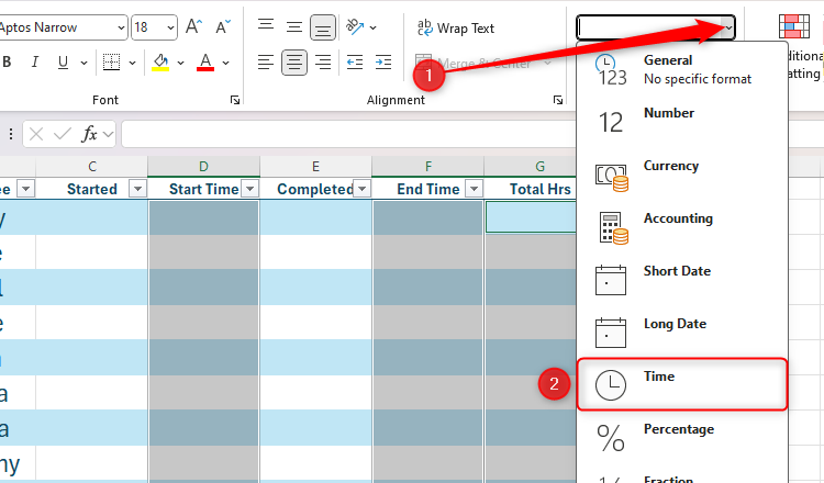
Now, in the Number group in the Home tab on the ribbon, click the “Number Format” drop-down menu, and select “Time.”
By default, Excel displays time in the HH:MM:SS format. To
change this time format
, click the “Number Format” drop-down menu again (with the relevant columns still selected), click “More Number Formats,” and choose a different time format from the options displayed. Alternatively, to display the time and date together, click “Custom” in the Format Cells dialog box, and type
dd/mm/yyyy hh:mm:ss
into the box at the top.
Step 3: Add Your Checkboxes
It’s now time to add checkboxes to the relevant columns. Select the first cell of a checkbox column in your table, and click “Checkbox” in the Insert tab on the ribbon. If you don’t see this option, instead type Checkbox into the search bar at the top of your window, and click “Checkbox.”
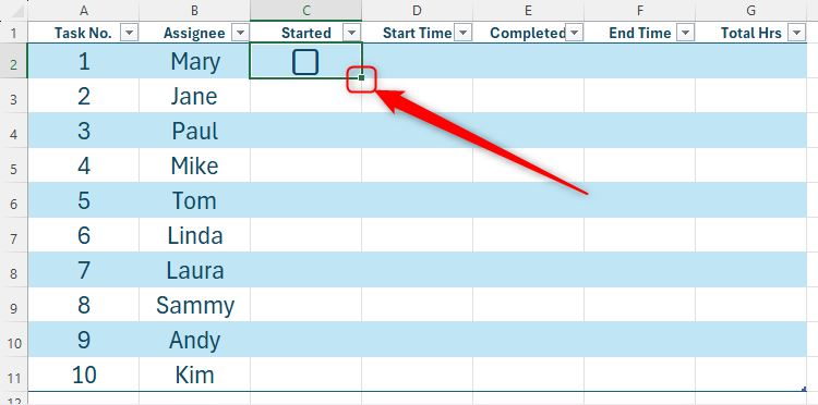
Next, select the cell containing the first checkbox, and double-click the fill handle in the bottom-right corner of that cell to fill the remaining cells in that column.
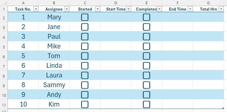
If you have more columns that also require checkboxes, repeat the above process or copy and paste the checkbox column you have already created.
Step 4: Enable Iterative Calculations
You’re now ready to prepare your spreadsheet for the timestamp calculation you’re going to add in the next step.
This calculation will be what’s known as an iterative formula, meaning it refers to itself within the formula (also known as a circular reference). If you use a simpler formula, the timestamp will continually update to the current time because the formula contains a volatile function (NOW). And if you don’t enable iterative calculations when using the method in this guide, Excel will return an error.
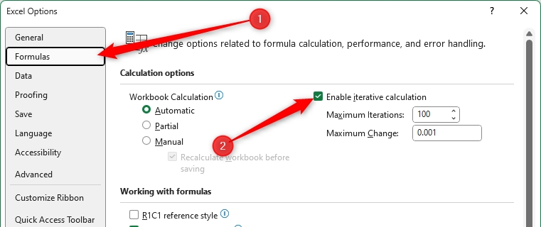
Press Alt > F > T to launch the Excel Options dialog box, and check “Enable Iterative Calculation” in the Formulas menu.
When you click “OK,” you won’t see any visible changes to your spreadsheet, but under the surface, it’s ready for the next step.
While useful in this scenario, it’s important to know some of the drawbacks of iterative calculations. For example, since they recalculate in a loop, they may affect your spreadsheet’s overall performance. Also, enabling this feature will mean that Excel doesn’t identify any incorrectly used circular references, so keep an eye on this. Finally, if you share the workbook with people using an older version of Excel, the timestamps may not work in the same way as on your version.
Step 5: Apply the Magic Formula
The final step is to create the formula to generate a timestamp when a checkbox is checked. I’m going to start with column D, which will produce a timestamp when I check a box in column C.
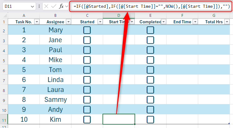
Here’s the formula that I will use in cell D2:
=IF([@Started],IF([@[Start Time]]="",NOW(),[@[Start Time]]),"")
While this looks complicated, when broken down, it makes more sense.
The first IF function evaluates whether the corresponding checkbox in column C (the Started column) is checked:
=IF([@Started],
Excel then moves to the second IF function, which evaluates whether the current cell (D2 in the Start Time column) is blank:
=IF([@Started],IF([@[Start Time]]="",
If it is blank, you want the current time to be inserted:
=IF([@Started],IF([@[Start Time]]="",NOW(),
If it is not blank, you want Excel to keep the cell as it is:
=IF([@Started],IF([@[Start Time]]="",NOW(),[@[Start Time]]),
The final argument will make sure that if the corresponding checkbox in column C isn’t checked, the value in column D will be blank:
=IF([@Started],IF([@[Start Time]]="",NOW(),[@[Start Time]]),"")
When you press Enter, the formula will be applied to the remaining cells in that column.
Now, copy and paste that formula into the first cell of any other column that requires timestamps based on checkboxes, and adjust the formula’s references so that it captures the correct columns.
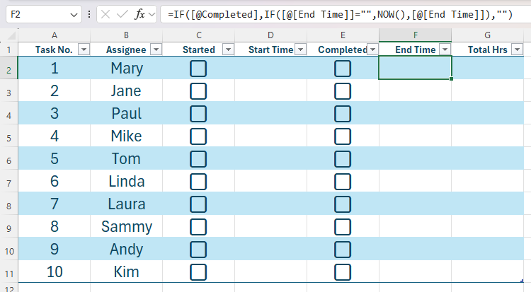
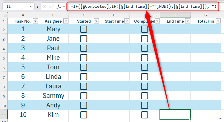
In my case, after pasting the formula into cell F2, I’ve changed the word “Started” (referencing column C) to “Completed” (referencing column E), and “Start Time” (referencing column D) to “End Time” (referencing column F):
=IF([@Completed],IF([@[End Time]]="",NOW(),[@[End Time]]),"")
When you do this for the first cell, it will apply automatically to the other cells in that column after you press Enter.
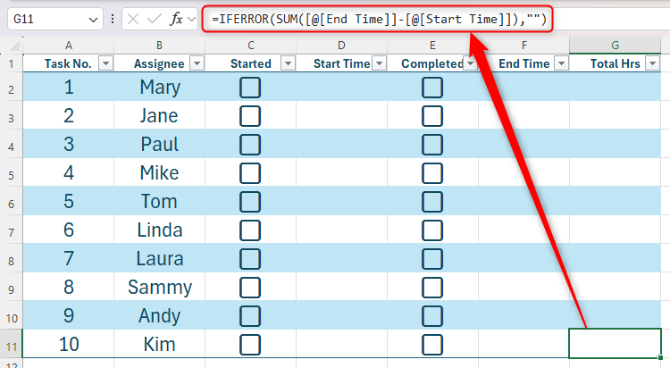
Finally, to use this data to calculate a total completion time, I will embed a simple SUM calculation within an IFERROR calculation in cell G2. This means that if the SUM doesn’t work because the checkboxes are unchecked, the corresponding cell in column G (Total Hrs) will remain blank:
=IFERROR(SUM([@[End Time]]-[@[Start Time]]),"")
Again, once I press Enter, the formula will be applied to all rows in that column.
Step 6: Try It Out!
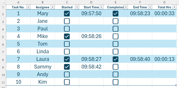
Before you put your checkboxes and timestamps to real-world use, check some of the checkboxes to make sure everything works as expected.
Adding conditional formatting rules to your checkboxes can make your data easier to read. For example, you can make cells containing checkboxes turn green when checked, or you could go one step further and format the whole row.
Source link


