How to Use the OFFSET Function in Excel

Excel’s OFFSET function lets you create a reference that is—quite literally—offset from a starting point. It allows references to adjust dynamically to changes in your spreadsheet’s data and structure.

The OFFSET Syntax

Before we look at how it works in practice, let’s run through the syntax. The OFFSET function has five arguments:

=OFFSET(A,B,C,D,E)

where

• A is the cell reference of the starting point,
• B is the number of rows to move down from point A,
• C is the number of columns to move right from point A,
• D (optional) is the number of rows (height) displayed in the result, and
• E (optional) is the number of columns (width) displayed in the result.

Values B, C, D, and E can be either numerical or cell references.

A Basic Example of OFFSET

To exemplify how OFFSET works, I’ll use a very basic, non-practical example. Typing

=OFFSET(A1,2,3,2,3)

into cell A6 would use cell A1 as the starting point (A), move down 2 rows (B), move across 3 columns (C), and return a series of values 2 cells high (D) and 3 cells wide (E):

If I had not typed values D and E in my formula, the result would have defaulted to referencing cell D3 (Deer) alone. This is because Excel assumes the result is the same size as the reference if you don’t specify the height and width.

Based on this principle, you can also define the size of the result within value A. For example, typing

=OFFSET(A1:A3,2,3)

would return a result that is three cells high, as this is the size of the starting point A.

Using OFFSET in the Real World

Now, I’ll show you how OFFSET can be used in real-world examples.

Real-world Example 1

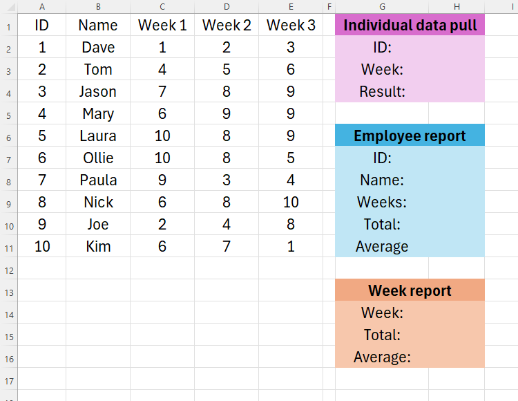
Here, I’ve got ten employees, and the number of units they’ve sold over three weeks. I’m going to use OFFSET to create three data reports.

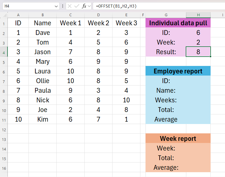
In the first data report (purple), I want Excel to tell me the number of units an employee has sold when I enter their ID and a week number. To achieve this, in cell H4, I’ll type

=OFFSET(B1,H2,H3)

where B1 is the starting point, H2 tells Excel how many rows down it needs to offset from the starting point (in other words, the employee ID), and H3 tells Excel how many columns across to offset from the starting point (in other words, the week number). Notice how I’ve used cell references here, because this means the data the OFFSET function pulls from my table can be dynamic.

After typing the above formula into cell H4, I’ll type 6 into the ID box (cell H2), and 2 into the week box (cell H3). This will tell me how many units Ollie sold in week 2, because the OFFSET function is pulling the data from the cell six rows down and two columns across from my starting point, cell B1.

I can now change the values in cells H2 and H3 at any point to pull any individual figure from the table.

Next, I want to create an employee report in the blue table. When I enter an employee ID, Excel will automatically tell me the employee’s name (using the VLOOKUP function), the total number of weeks of data we have (using the COUNTIF function), and the total and average units sold by that employee (using SUM and AVERAGE with OFFSET).

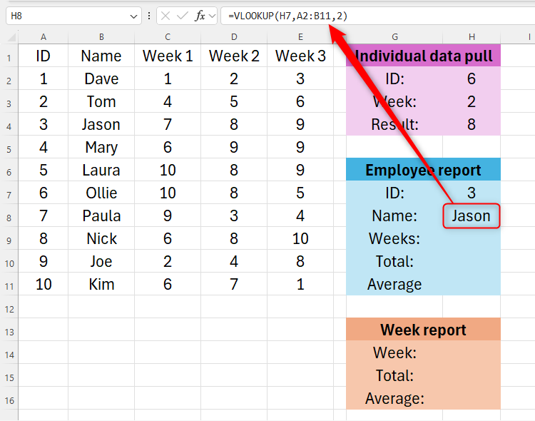
First, I will type an employee ID into cell H7 to get us started. Let’s go for employee ID 3, which is Jason. Then, I’ll use the VLOOKUP function to return Jason’s name in cell H8:

=VLOOKUP(H7,A2:B11,2)

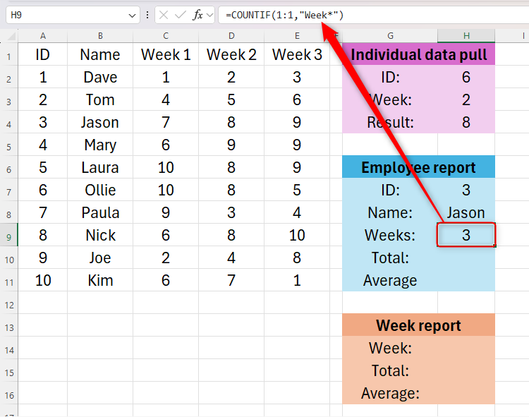
Now, I’ll use the COUNTIF function with a wildcard to tell Excel to count how many cells in row 1 contain the word “Week” followed by a number:

=COUNTIF(1:1,"Week*")

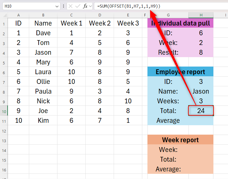
I can now use this information to work out Jason’s total and average units sold. First, in cell H10, I’ll type

=SUM(OFFSET(B1,H7,1,1,H9))

where B1 is my starting point, H7 is the number of rows to offset downwards (employee ID), the first 1 is the number of columns to offset to the right, the second 1 is the height of the result, and H9 is the width of the result (the total number of weeks). However, because OFFSET is embedded within the SUM function, the result will only be a single cell in size.

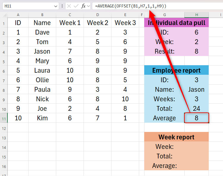
I can copy and paste the same formula into cell H11, but change SUM to AVERAGE, since I’m using the same references.

=AVERAGE(OFFSET(B1,H7,1,1,H9))

I can now change the value in cell H7 to generate a report for any other employee in my data table. What’s more, if I were to add another week to my data, cell H9 would automatically change to 4, and the subsequent calculations in cells H10 and H11 would also update.

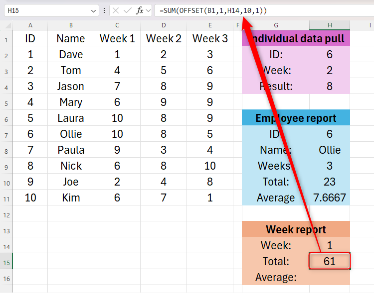
Finally, I want to create a weekly report in the orange table. This will require me to input a week number, and Excel will then generate the total and average units sold for that week. I’ll start by typing 1 into cell H14, so Excel will produce data from week 1. Then, in cell H15, I’ll type

=SUM(OFFSET(B1,1,H14,10,1))

where B1 is the starting point, the first 1 is the number of rows to offset downwards, H14 is the number of columns to offset to the right (week number), 10 is the height of the result, and the second 1 is the width of the result. However, because OFFSET is embedded within the SUM function, the result will only be a single cell in size.

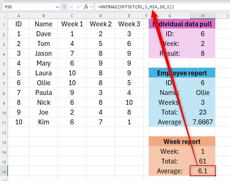
Finally, I can copy and paste that formula into cell H15, and change SUM to AVERAGE.

=AVERAGE(OFFSET(B1,1,H14,10,1))

Real-world Example 2

In this example, I’ll show you how to use OFFSET with a formatted table, and what it looks like when used to return a result in more than one cell.

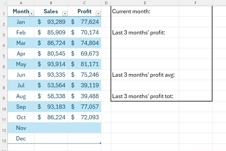
Here, I have current sales and profits so far this year in a formatted table, and I want my report table on the right to display the last three months’ profit totals individually, as well as the average and total profit for the same period.

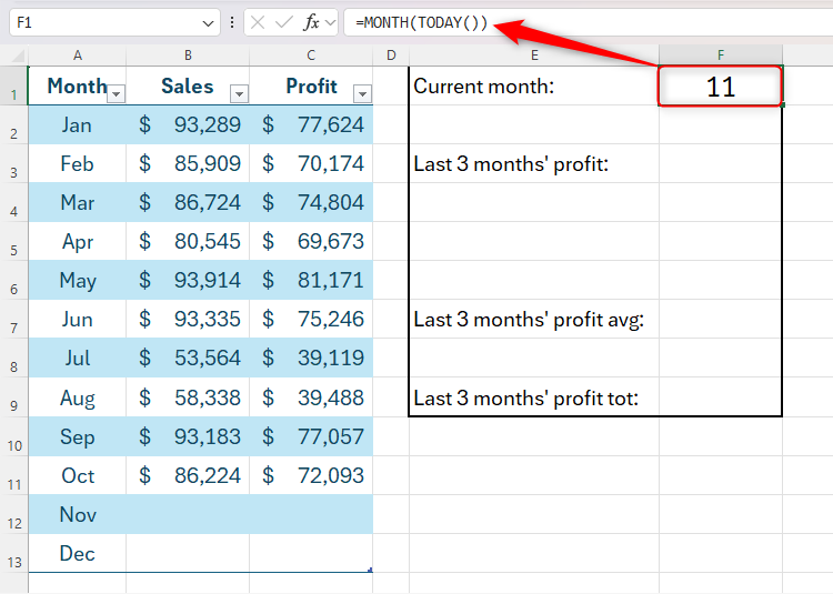
First, I need Excel to work out how many full months have elapsed so far, so that when I use OFFSET, I can use this figure to tell Excel how far from the starting point I need to offset. To do this, in cell F1, I’ll type

=MONTH(TODAY())

which will display the current month number. In this case, it’s November, month 11.

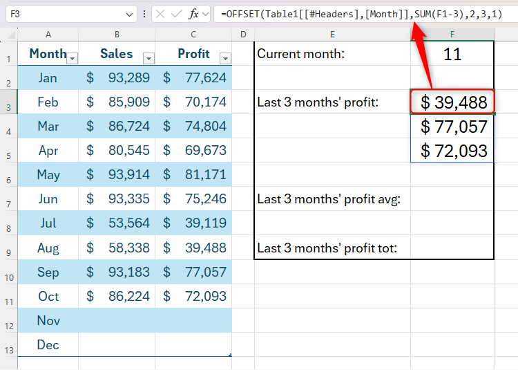
We can now use this month number to display the profits from the past three months. In cell F3, I’ll type

=OFFSET(

and click cell A1, my starting point. This will automatically add the formatted table’s month column header into the formula:

=OFFSET(Table1[[#Headers],[Month]]

Now, I’ll add a comma, and continue my OFFSET formula. The next stage is to tell Excel how many rows to offset downwards. This will be the current month (cell F1) minus three:

=OFFSET(Table1[[#Headers],[Month]],SUM(F1-3),

Finally, I’ll tell Excel that we need to offset two columns to the right, and the result will be three rows high and one column wide.

=OFFSET(Table1[[#Headers],[Month]],SUM(F1-3),2,3,1)

Notice how cells F4 and F5 contain data, even though the formula is only in F3. This is known as a spilled array, because the data has spilled over the active cell.

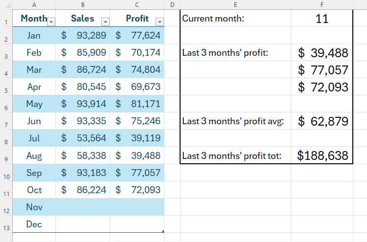
Now, when the month changes to 12 (December), Excel will automatically move this result down one cell, because the value in cell F1 will have increased by one.

I can then complete my table by typing

=AVERAGE(F3#)

into cell F7, and

=SUM(F3#)

into cell F8.

Things to Remember

There are two important things to remember when using OFFSET:

1. OFFSET is a volatile function, meaning it’s always looking to update. This could cause performance issues if used in an especially large spreadsheet or on a low-memory computer.
2. All the examples above are used to illustrate the different ways you can use the OFFSET function. There may be other, more efficient ways for you to create the same outcomes, such as by using the INDIRECT function. However, once you’ve understood how the functions work, you can decide which is best to use in your situation!

Personally, I use the OFFSET function to record and analyze my favorite football team’s data. After all, Excel isn’t just for accountants—you can use it at home alongside your hobbies!