How to Use the SEQUENCE Function in Excel

Excel’s SEQUENCE function lets you create a list of numbers in a sequence in an instant. It also allows you to define the shape, number of values, and steps between each number in the sequence, and you can use SEQUENCE in conjunction with other Excel functions.

The SEQUENCE Syntax

The SEQUENCE function has four arguments:

=SEQUENCE(a,b,c,d)

where

• a (mandatory) is the number of rows that the sequence will span (downwards),
• b (optional) is the number of columns it’ll span (across),
• c (optional) is the starting number in the sequence, and
• d (optional) is the increment between each value in the sequence.

Arguments a and b (the size of the resultant array) must be whole numbers (or formulas that output a whole number), while arguments c and d (the starting number and the increment in the sequence) can be either whole or decimal numbers. If argument d is 0, the result will repeat the same number, as you’re telling Excel not to add any increments between each value in the array.

If you choose to omit any of the optional arguments (b, c, or d), they will default to 1. For example, typing

=SEQUENCE(2,,10,3)

will return a sequence that is one column in height, since argument b is missing.

SEQUENCE is a dynamic array formula, meaning it can produce a spilled array. In other words, although the formula is typed into one cell, if arguments a or b are greater than 1, the result will spill over to more than one cell.

How the SEQUENCE Function Works

Before I show you some variations and real-world uses of SEQUENCE, here’s a straightforward example that demonstrates how it works.

In cell A1, I typed

=SEQUENCE(3,5,10,5)

meaning the sequence is three rows in height and five columns wide. The sequence starts with the number 10, and each subsequent number is an increment of five from the previous one.

Filling Down Then Across: TRANSPOSE

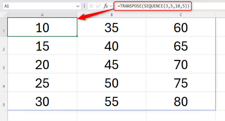
In the example above, you can see that the sequence first fills across the columns, and then down the rows. However, by embedding the SEQUENCE function within the TRANSPOSE function, you can force Excel to fill the numbers down the rows, and then across the columns.

Here, I typed the same formula as in the example above, but I also embedded it within TRANSPOSE.

=TRANSPOSE(SEQUENCE(3,5,10,5))

As a result, Excel flipped arguments a and b in the syntax, meaning the “3” now represents the number of columns, and the “5” represents the number of rows. You can also see that the numbers fill down and then across.

Creating a Sequence of Roman Numerals

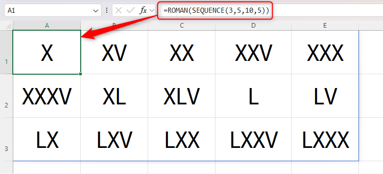
If you want to create a sequence of Roman numerals (I, II, III, IV) instead of Arabic numbers (1, 2, 3, 4), you’ll need to embed your SEQUENCE formula within the ROMAN function.

Using the same parameters as in the example above, I typed

=ROMAN(SEQUENCE(3,5,10,5))

into cell A1 to produce this result:

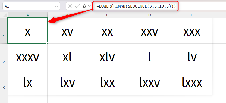
Going one step further, suppose I wanted the Roman numerals to be lowercase. In this scenario, I would embed the whole formula within the LOWER function.

=LOWER(ROMAN(SEQUENCE(3,5,10,5)))

Using SEQUENCE to Create Dates

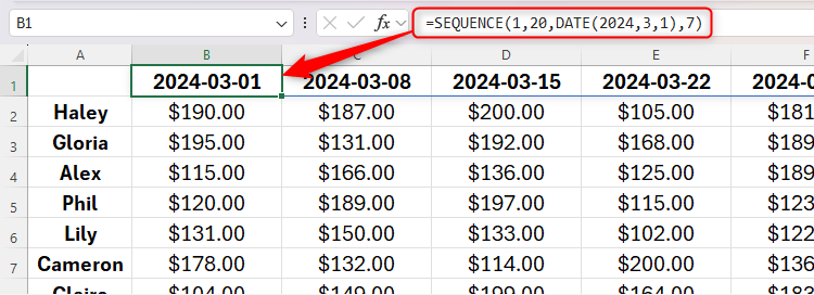
A more practical use of the SEQUENCE function is to generate a sequence of dates. In the example below, I wanted to create a report that contained each person’s weekly profit, starting on Friday, March 1st, and continuing each Friday for 20 weeks.

To do this, I typed

=SEQUENCE(1,20,DATE(2024,3,1),7)

into B2, because I wanted the dates to run across the first row for 20 columns, starting Friday, March 1st, and incrementing seven days from one value to the next.

Making SEQUENCE Depend on Another Parameter

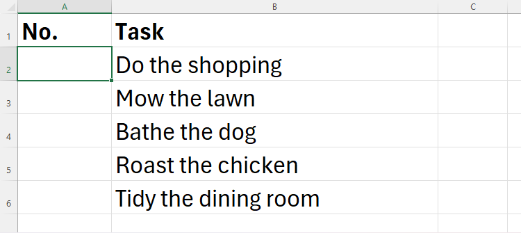
In this example, I have a list of tasks that need to be numbered. I want Excel to automatically add another number when I add another task (or, by the same token, remove a number when I complete and delete a task).

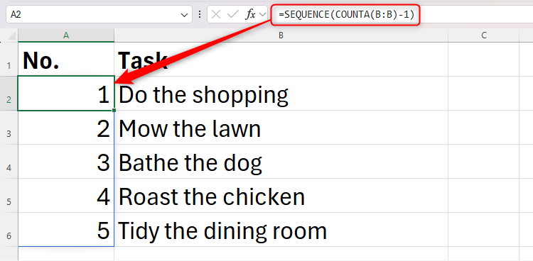
To do this, in cell A2, I typed

=SEQUENCE(COUNTA(B:B)-1)

The number of rows the sequence fills now depends on the number of cells in column B that contain text (thanks to the COUNTA function), and I added “-1” to the end of the formula so that the COUNTA calculation discounts the heading row.

You’ll also notice that I only specified argument a (the number of rows) within my SEQUENCE formula, because leaving all the other arguments out defaults them to 1, which is what I want in this example. In other words, I want the result to only occupy one column, the numbering to start at 1, and the sequence to increase by one each time.

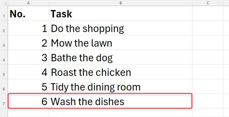
Now, when I add an item to the list in column B, the numbering in column A updates automatically.

Things to Note When Using SEQUENCE

There are three caveats to be aware of when using the SEQUENCE function in Excel:

1. Dynamic array formulas that produce spilled arrays—including SEQUENCE—cannot be used within formatted Excel tables. The best fix if you want to use SEQUENCE among existing data is to convert your formatted Excel table to an unformatted range by selecting one of the cells within the table, and clicking “Convert To Range” in the Tools group of the Table Design tab.
2. If you create dynamic arrays linking two workbooks, this will only work if both workbooks are open. As soon as you close the source workbook, the dynamic array formula in the active workbook will return a #REF! error.
3. Interrupting a spilled array by placing another value in an affected cell will break your SEQUENCE function and result in the #SPILL! error.

Why Use SEQUENCE Instead of the Fill Handle?

An alternative to the SEQUENCE function is Excel’s fill handle, which you can click and drag to continue a sequence you have already started:

However, there are several reasons why I prefer to use the SEQUENCE function instead:

• If you want to create a long sequence, dragging can take forever!
• It is easier to amend the parameters of the sequence within the SEQUENCE function—simply adjust the arguments within your formula. When you click and drag the fill handle, you have to remember to select more than one number in the existing array.
• If you delete rows or columns that interact with your sequence, numbers created through the fill handle will also be deleted. However, since SEQUENCE results in a spilled array, they stay put, even when you restructure your spreadsheet.
• Excel’s fill handle is designed to fill a sequence along a single row or column. To create a sequence using the fill handle that covers numerous rows and columns, you have to take more steps than when you use the SEQUENCE function, which allows you to specify all your parameters in one go.
• The SEQUENCE function removes any human error that might occur when using the fill handle.

If you use SEQUENCE with a volatile function, such as DATE, this could cause your Excel workbook to slow considerably, especially if you already have lots of data in your spreadsheet. So, try to limit the number of volatile functions you use to ensure your Excel sheet works quickly and effectively.