Microsoft Excel has hundreds of tools that you can use to make your spreadsheets tick. However, if you’re looking to level up your expertise, get to know these six essential features today.
This is a whistle-stop tour of some must-know tools in Microsoft Excel. To find out more about each feature, click the “Related” links in each section.
6
Excel Tables for Data Organization
A Microsoft Excel worksheet is essentially a large table organized into columns and rows, with each column-row intersection forming a cell where you can enter data or formulas. Within that larger structure, however, you can create mini datasets that work independently.
This is where Excel tables come into play. They come with built-in filtering and sorting capabilities, expand with new data, duplicate formulas down a whole column, and allow you to quickly add a total row for instant data analysis. What’s more, you can use table column headers in formulas—also known as structured references—as well as choose from various table formatting options.
Related
Everything You Need to Know About Excel Tables (And Why You Should Always Use Them)
This could totally change how you work in Excel.
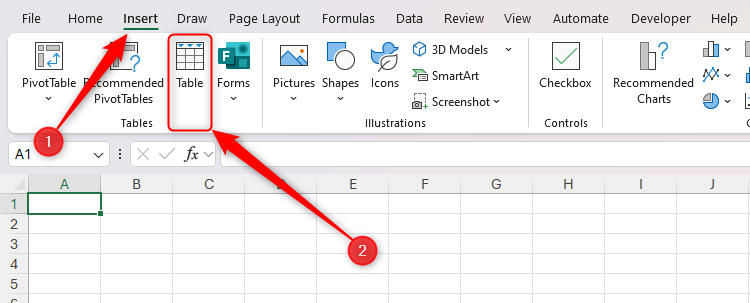
If you’re starting with a blank canvas, click “Table” on the Insert tab on the ribbon.
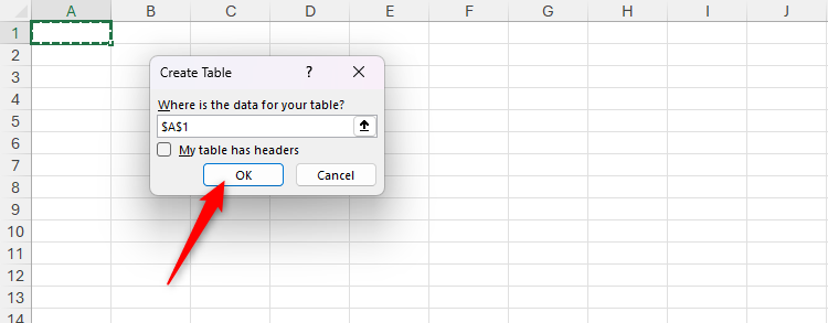
Then, click “OK” in the Create Table dialog box.
Within the newly created table, rename the first column, and start inputting your data.
As soon as you type in the first blank cell beneath the table and press Enter, the table automatically grabs that cell and includes it as part of the dataset. Similarly, adding values to the first blank column next to the table expands the formatting to the right.
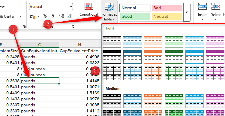
If you already have your dataset and want to convert it into a formatted table, select any cell within the range, and in the Home tab on the ribbon, click “Format As Table,” and choose a style.
Next, if your table has headers, check this option in the Create Table dialog box. If it doesn’t, leave this option unchecked, and Excel will add a header row for you.
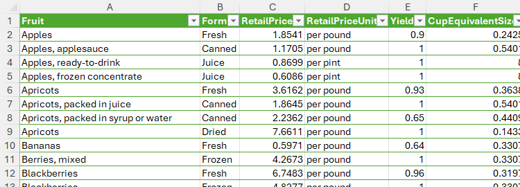
When you click “OK,” your data is instantly transformed into a tidily presented table.
If your dataset contains formulas that reference other columns within the range, you’ll need to recreate these using structured references once you’ve formatted the data as an Excel table. In other words, if a formula reads =SUM(A2+B2), delete A2 and B2, and replace these direct references with column references by clicking the relevant cells.
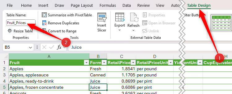
Whether you’re starting from scratch or converting a pre-existing dataset into a formatted table, an important step to take is naming your table. This means that it can be referenced in formulas outside the table, and you can jump to it at any point via the name box in the top-left corner of the Excel window.

Related
If You Don’t Rename Tables in Excel, Today’s the Day to Start
What’s in a name? Well, quite a lot.
To do this, select any cell within the table, and in the Table Design tab, head to the “Properties” group, and type a new name.
The Table Design tab is where you can change how your table looks and behaves. You can adjust the overall layout of the table in the Table Styles group, and you can choose whether to include elements like a total row or banding in the Table Style Options group. What’s more, you can add slicers to your table to make it easier to filter your data.
If you’ve never used Excel tables before, you’ll be amazed at just how much easier they make data management and organization.
5
Lookup Functions for Cross-Referencing
I probably use lookup functions in my Excel spreadsheets more than any other type of function. They’re a powerful and efficient way to look up a value in a dataset, and return a corresponding result.
Microsoft lists 36 lookup and reference functions, but XLOOKUP and INDEX with MATCH are the most useful for day-to-day data referencing. Let me show you some examples.
Example 1: Returning a Value in a One-Dimensional Lookup
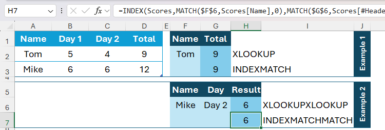
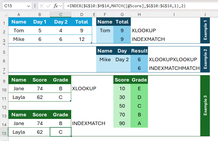
In this straightforward example, the aim is to use these functions to return the total score of the player whose name is typed in cell F2.
To do this in cell G2 using the XLOOKUP function, you need to type:
=XLOOKUP($F$2,Scores[Name],Scores[Total])
where
- $F$2 is the cell containing the value to look up (in this case, Tom),
- Scores[Name] tells Excel to look for this value in the Name column of the table named “Scores,” and
- Scores[Total] returns the corresponding value from the Total column of the Scores table.
When you press Enter, the lookup correctly returns a total score of 9.

Related
Forget VLOOKUP in Excel: Here’s Why I Use XLOOKUP
Out with the old, and in with the new.
To get the same result using the INDEX and MATCH functions, in cell G3, you need to type:
=INDEX(Scores[[Day 1]:[Total]],MATCH($F$2,Scores[Name],0),3)
where
- Scores[[Day 1]:[Total]] is the array containing the value you want to return,
- MATCH($F$2,Scores[Name],0 takes the value in F2, and returns the row number of the corresponding value in the Name column of the Scores table, and
- 3 returns the value in the array that is in the third column of that row.

Related
How to Use INDEX and MATCH in Microsoft Excel
When VLOOKUP doesn’t cut it, you have another option for lookups in your spreadsheet.
Notice how, when comparing these examples, the XLOOKUP formula is much more straightforward. XLOOKUP was introduced to Excel later than INDEX and MATCH, so it’s a more refined way to complete this one-dimensional lookup task.
Example 2: Returning a Value in a Two-Dimensional Lookup
XLOOKUP and INDEX with MATCH can also perform two-way lookups. In this example, in cells H6 and H7, you want to use these functions to return a player’s score on a particular day, depending on the name in cell F6 (in this case, Mike) and the day in cell G6 (in this case, day 2).
To do this in cell H6 using XLOOKUP, you need to type:
=XLOOKUP($G$6,Scores[[#Headers],[Day 1]:[Total]],XLOOKUP($F$6,Scores[Name],Scores[[Day 1]:[Total]]))
where the first XLOOKUP looks up the value in cell G6 across the column headers, and the second XLOOKUP looks up the value in cell F6 in the Name column. Then, it returns the result from the array.
Using INDEX and MATCH, in cell H7, type:
=INDEX(Scores,MATCH($F$6,Scores[Name],0),MATCH($G$6,Scores[#Headers],0))
where the INDEX part of the formula identifies the array containing the value to return, the first MATCH looks up the value in cell F6 in the Name column, and the second MATCH looks up the value in G6 across the column headers.
In this case, the formula when using the INDEX-MATCH-MATCH combination is shorter than the formula when using XLOOKUP-XLOOKUP, so I would tend to use the former for two-dimensional lookups.
Example 3: Using Lookup Functions in a Table
In the examples above, the lookups were performed outside the main data tables. However, you can also use these functions within a formatted Excel table.
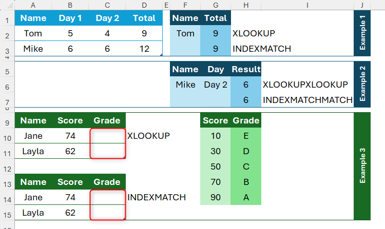
In example 3, your aim is to return the students’ grades based on their scores.
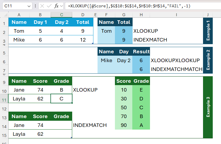
To do this using XLOOKUP, in cell C10, type:
=XLOOKUP([@Score],$G$10:$G$14,$H$10:$H$14,"FAIL",-1)
where
- [@Score] takes each student’s score,
- $G$10:$G$14 tells Excel to look for each score in those cells,
- $H$10:$H$14 is the value to be returned (in this case, a grade) in the active cell,
- “FAIL” is what to return if the lookup value cannot be found, and
- -1 tells Excel to look for exact matches or return the next smallest item.
When you press Enter, the formula is duplicated automatically to the remaining cells in the column.
To do this using INDEX and MATCH, in cell C14, type:
=INDEX($G$10:$H$14,MATCH([@Score],$G$10:$G$14,1),2)
where
- $G$10:$H$14 is the range where the lookup values are located,
- MATCH([@Score],$G$10:$G$14 matches the score in the Grade column to the scores in the lookup table,
- 1 finds the largest value that is less than or equal to the lookup value, and
- 2 tells Excel to look in the second column for the result.
Then, press Enter to commit the formula and apply it to the other cells in that column.
Both XLOOKUP and INDEX with MATCH require five arguments, and their formulas are of similar lengths. However, since XLOOKUP allows you to specify what to return if the value cannot be found, it’s my go-to in these scenarios.

Related
INDEX and MATCH vs. VLOOKUP vs. XLOOKUP in Microsoft Excel
Which is the best for finding data?
4
Conditional Formatting for Instant Data Visualization
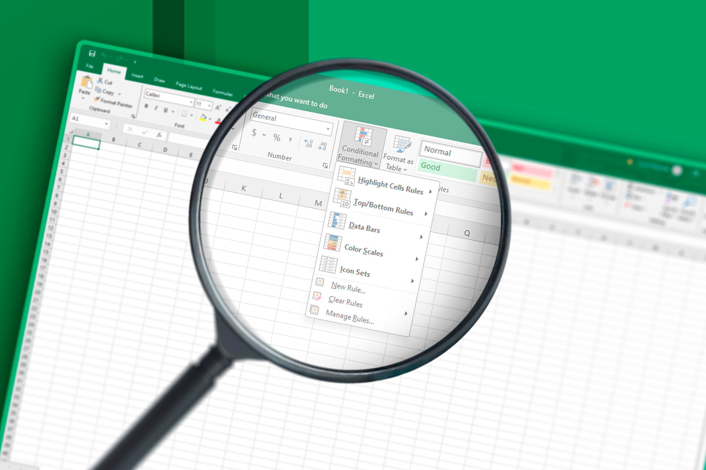
You might know how to use all the complex Excel formulas in the book, but that’s no good if the figures they produce aren’t easy to read. That’s why conditional formatting is an essential tool to use in every spreadsheet. It does what its name suggests—formats cells based on certain conditions.
Related
I Use Conditional Formatting in Most Spreadsheets: Here’s Why
Conditional formatting is a non-negotiable.
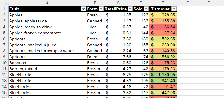
Imagine you own a grocery store, and you want to clearly visualize how much money you have made on each fruit.
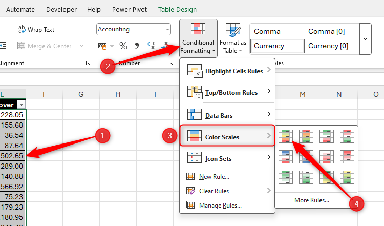
Yes, you can see the figures in column E, but they’re currently not particularly easy to interpret. To fix this, select the data in the column by clicking the black arrow that appears when you hover over the column header, and in the Home tab on the ribbon, click the “Conditional Formatting” drop-down menu, hover over “Color Scales,” and choose the green-to-red option.
Now, you can instantly see which figures are higher, and which figures are lower.

Related
How to Apply a Color Scale Based on Values in Microsoft Excel
Visualize your Excel data in an instant.
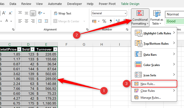
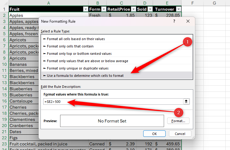
You can also use conditional formatting to set more specific rules. For example, instead of coloring column E using color scales, you want to highlight the whole row of any fruit that has made over $500. To do this, select the highest left-most cell beneath the column headers, and press Ctrl+A to select the whole range. Then, click Conditional Formatting > New Rule.
Now, in the New Formatting Rule dialog box, click “Use A Formula To Determine Which Cells To Format,” and in the text field, type:
=$E2>500
This takes all the cells in column E, starting at cell E2, and evaluates their values to see whether they’re greater than 500.
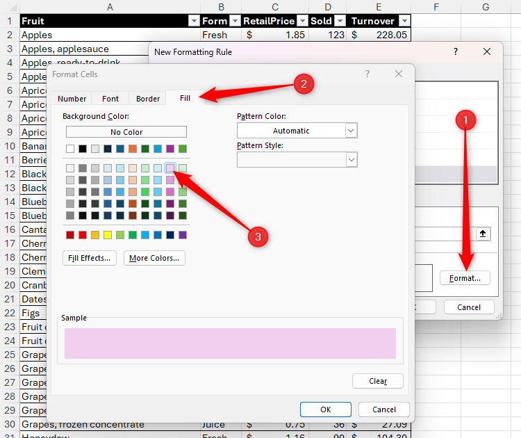
Finally, click “Format” to choose a cell style that will be applied when the above criterion is met. In this case, I’m going for a lilic cell fill.
Click “OK” to close the dialog boxes and complete the process.
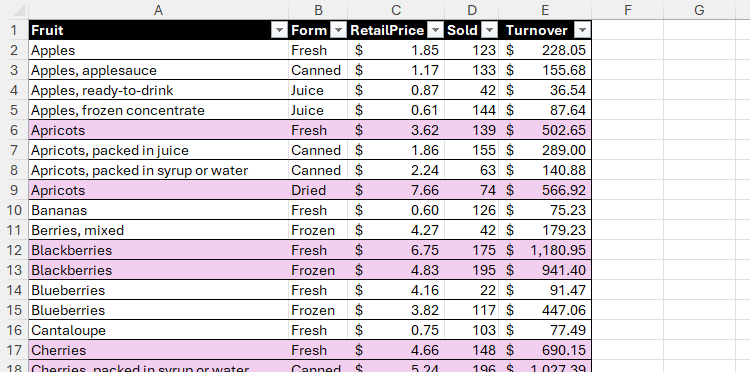
Because you selected all the columns in the first step, the whole row for each qualifying value is now highlighted.
Conditional formatting can be used to apply formats in many different contexts, including formatting certain dates, or applying formatting if a cell’s value is above or below the average.

Related
How to Highlight Values Above or Below Average in Excel
Spot those high or low values at a glance.
3
Data Validation for Consistency and Error Prevention
Whether you plan to share your spreadsheet with others, or keep it for your own use, data validation is a great tool for ensuring cells contain the values or types of values you expect. As a result, it ensures consistency, helps prevent typos, and saves time.
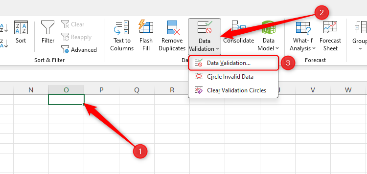
First, select the cell or cells to which you want to apply the data validation rule, and in the Data tab on the ribbon, click “Data Validation.” If you see a drop-down menu, click “Data Validation” again.
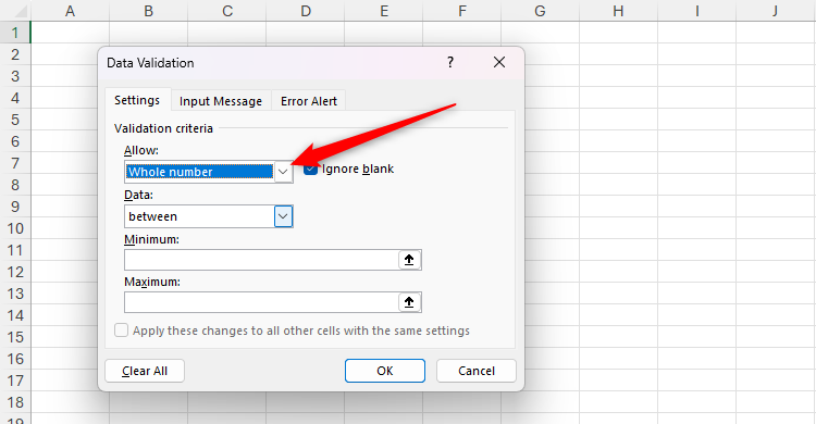
By default, any value can be entered into a cell in Excel. However, if you expand the “Allow” drop-down menu of the Data Validation dialog box, you can see the types of restrictions you can apply. For example, if you select “Whole Number,” “Decimal,” “Date,” “Time,” or “Text Length,” you’re given the option to specify the parameters for those data types.

Related
How To Restrict Data Input In Excel With Data Validation
Take control over the data in your worksheet.
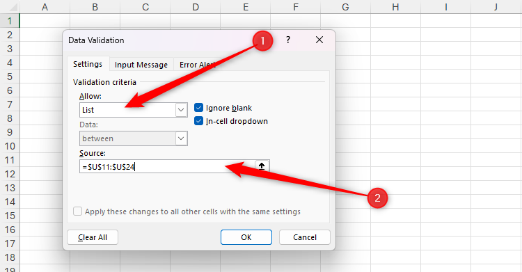
On the other hand, if you select “List,” you can either type a list of allowed values (separated by commas) in the Source field, or reference cells containing the allowed values.
After you click “OK,” a drop-down button appears when the affected cell is selected, which you can click to reveal the entry options.

Related
How to Add a Drop-Down List to a Cell in Excel
It beats typing in the same options 200 different times manually.
Finally, the Data Validation dialog box has two other tabs, where you can further refine the validation cleanliness of the selected cells:
- Input Message: This tab lets you create a message that appears when the cell is selected. This is a good way of reminding whoever is inputting data that only certain values are permitted in that cell.
- Error Alert: In this tab, you can create a message that appears when the wrong data type is inputted into the cell.
2
Power Query for Data Manipulation
Power Query is an underestimated tool that everyone—from Excel novices to power users—can and should use. It allows you to import and connect datasets from various sources, including the web, PDFs, and separate worksheets within a workbook, as well as manipulate the data to meet your needs.
For example, you can split cells into two or more new cells, replace errors with more meaningful values, unpivot data to aid analysis, fill blank cells based on the cell above, and much more. You can also stack tables that have the same column headers from various worksheets.

Related
4 Excel Power Query Commands You Need to Know
Become an expert data manipulator.
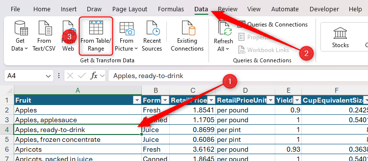
To transform existing data in your worksheet, select any cell in the range in question, and in the Data tab on the ribbon, click “From Table/Range.”
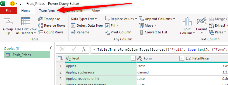
The Power Query Editor then opens, where you can begin your data manipulation. The Transform tab is where most of the magic happens, so this is a good place to start. Right-clicking the column headers also gives you access to many column-specific tools.
Related
How to Clean Up and Import Data Using Power Query in Excel
Don’t overlook this amazing Excel tool!
When you’ve finished editing your data, click “Close And Load” in the Home tab on the ribbon to send the dataset to a new worksheet in your workbook.
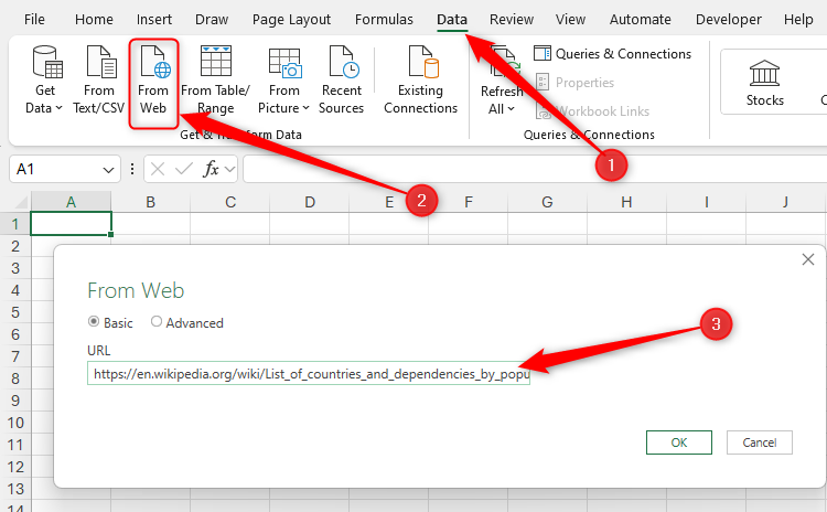
To import a table from a website, head back to the “Data” tab on the main Excel ribbon, click “From Web,” and paste the URL into the text field of the window that appears.
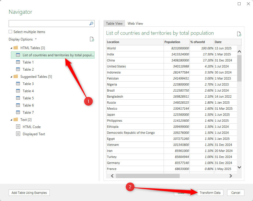
When you click “OK,” the Navigator dialog box appears, where you can select the table you want to import and edit, before clicking “Transform Data” to open the Power Query Editor.

Related
How to Import Tables From the Web to Excel 365
Don’t waste time or risk errors by copying data manually.
1
Wildcards for Partial Matches
Wildcards in Excel represent unknown or non-specific characters in searches, filters, and formulas.
There are two types of wildcards you can use to identify values with fuzzy matches:
- The asterisk (*): This represents any number of characters (including no characters). For example, “OK*” would return a match for “Oklahoma,” but not for “look.”
- The question mark (?): This represents a single character. For example, “?OK” would return a match for “wok,” but not for “Joke.”
- Mixed wildcards: You can also combine the asterisk and question mark to further refine your search. For example, “*OK?” would return a match for “Books,” but not for “Took.”

Related
How You Can Use Wildcards in Microsoft Excel to Refine Your Search
Find partial matches in an instant.
If you want to search for question marks or asterisks as characters in their own right, place a tilde (~) before either symbol to cancel their wildcard functionality.
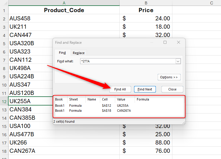
Wildcards are most commonly used when searching for certain values in Excel. In this example, after pressing Ctrl+F to launch the Find tab of the Find And Replace dialog box, typing *2??A returns two results from the dataset: UK255A and CAN267A.
Using the same dataset, you can use wildcards within the SUMIF function to add the prices of goods that come from the UK:
=SUMIF(A2:A18,"UK*",B2:B18)

Related
How to Use SUMIF in Microsoft Excel
Do you want to add numbers, but only if they meet your conditions? Use SUMIF!
Wildcards and text values must always be enclosed within quotation marks in formulas in Excel.
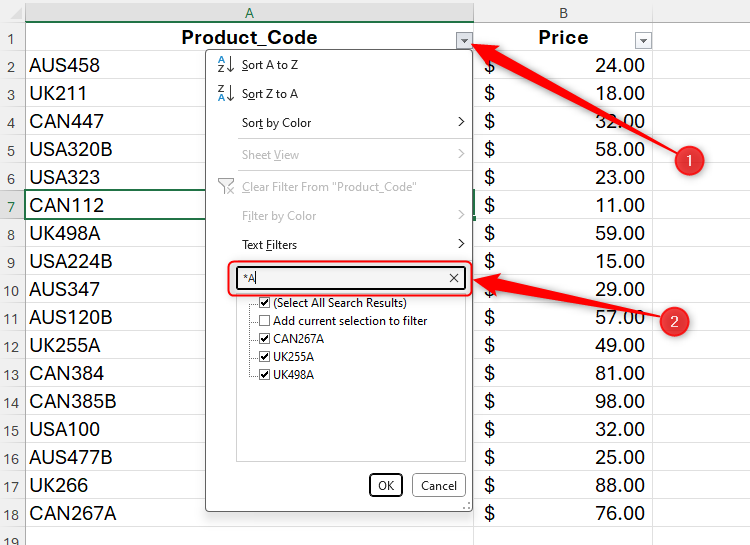
Finally, after pressing Ctrl+Shift+L to add filter buttons to the dataset, clicking the filter button at the top of column A and typing:
*A
into the text field returns all product codes ending in “A.”
Once you’ve got to grips with these essential tools, test your knowledge by taking on the How-To Geek beginner, intermediate, and advanced Microsoft Excel skills tests.
Source link


