4 Excel Power Query Commands You Need to Know

Have you heard of Power Query in Microsoft Excel but always thought that it’s only intended for Excel experts? Let me stop you there because, actually, Power Query is designed to be user-friendly and, most importantly, save you a lot of hassle when organizing your data.

This guide is intended for readers who are new to Microsoft Excel or Power Query. The tips don’t require you to know or use any Power Query M formula language, and they offer a good starting point for getting to know some of the commands you can use in this powerful data manipulation tool.

1

Split Cells by Delimiter to Isolate Values

There are many ways in Excel to split data into more than one column, including the Text To Columns tool, Flash Fill, and built-in functions. However, the most intuitive method is to launch the Power Query Editor, and perform the operation there.

Let’s imagine that you’ve found a table on Wikipedia that you want to transform using Power Query. To import the table, first, you clicked “Get Data” on the Home tab on the ribbon, and then selected From Other Sources > From Web.

Next, after pasting the URL into the text field in the From Web dialog box and clicking “OK,” you selected the table in the Navigator’s left-hand pane, and clicked “Transform Data.”

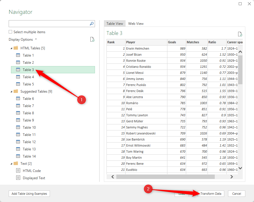
When the table loaded in the Power Query Editor, you noticed that the Career Span column contains two pieces of data—the year each player started their career, and the last year in which they played—and you want these to be in separate columns.

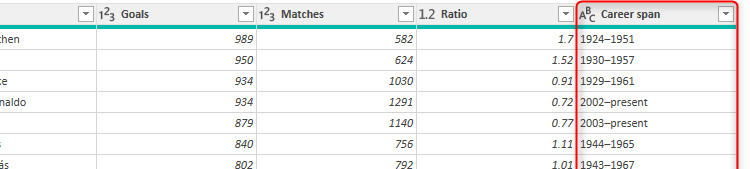
To do this, right-click the column header, hover over “Split Column,” and select “By Delimiter.”

A delimiter is a character, symbol, or space that is used to separate items in a sequence.

At this point, the Power Query Editor reviews the data in the column to see whether it can detect a potential delimiter. In this case, it’s identified that each cell contains a dash, and correctly assumes that this is the point at which the cell should be split. However, you can select a different delimiter from the first drop-down menu if necessary.

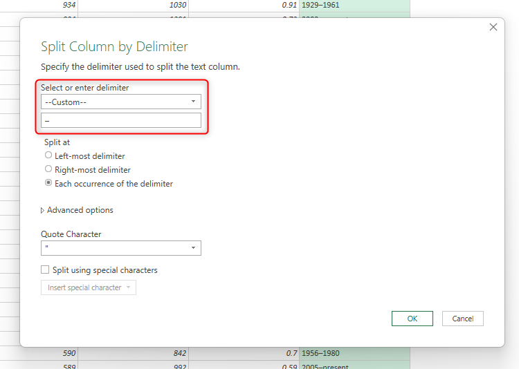
Since there’s only one delimiter in each cell of the selected column in this example, there’s no need to make any further changes to the options in the dialog box, so click “OK,” and see the newly transformed data in the Power Query Editor.

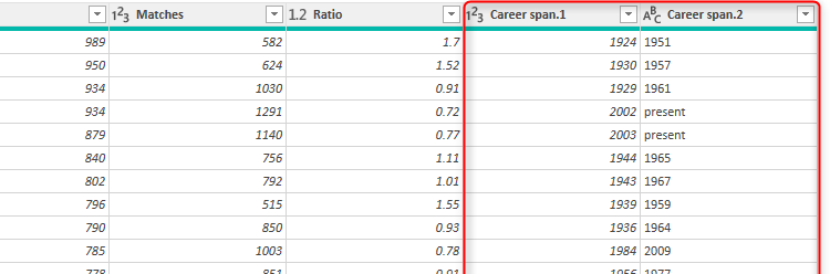
To rename the new columns, double-click the column headers, and type the new data labels.

Now, you’ve successfully split the data using the Power Query Editor, but did you notice that the cells in the two new columns are aligned differently? This is because the values in the “First played” column are all numbers (as indicated by the 123 icon next to the column header), but since the values in the “Last played” column include both text and numbers, Excel treats this as a text column (hence the ABC in the column header).

To fix this, select the “ABC” icon in the “Last played” column, and click “Whole Number.”

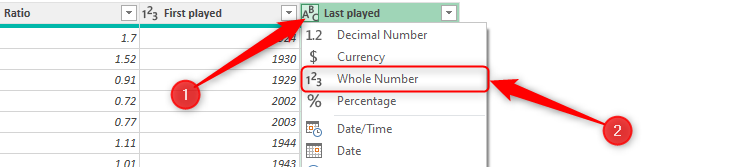
Now, both columns are formatted as numerical datasets.

However, because some cells in the “Last played” column contained text values, these now show as errors. But don’t fret—continue reading to find out how to fix this!

2

Replace Errors for Use in Calculations

Excel’s Power Query is a powerful tool for dealing with any errors that appear in your data.

Taking the query in the previous example, some cells in the “Last played” column contain errors, because they previously contained the text value “Present” in a column formatted as whole numbers.

At present, if you click “Close And Load” in the top-left corner of the Power Query Editor, those cells with error values will be blank in the resultant table. While this might seem ideal, blank cells in an Excel column can cause issues when you’re sorting and filtering the data or referencing column headers in formulas, so it’s best to fill them with meaningful values.

To do this, right-click the column header, and select “Replace Errors.”

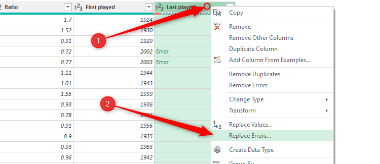
You might be tempted to select “Remove Errors” in the right-click menu. However, this deletes the entire row, not just the error, so only click this option if that’s what you want to happen.

Now, in the Replace Errors dialog box, type the value you want to appear instead of errors. In this case, since the errors appeared where the cell read “Present,” you could type the current year.

When you click “OK,” all the error values are replaced with this new value.

Because all the cells in the two right-most columns all contain the same data types without any errors, you can create a new column that works out the total number of playing years for each player.

Here, I clicked “Custom Column” in the Add Column tab, changed the column name to “Years played,” and used the list of columns in the Available Columns menu to create a simple subtraction.

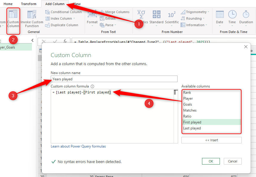
Then, when I clicked “OK,” this new column—free of any errors—was added to the right-hand side of the query.

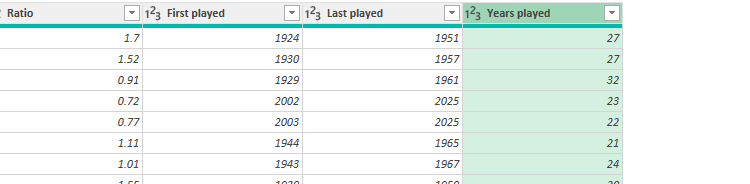
When you’re done, click the “Close And Load” icon in the Home tab of the Power Query Editor to send the table to a new spreadsheet in your Excel workbook.

3

Unpivot Data to Aid Analysis

When creating a new dataset in Microsoft Excel, where possible, I follow the record-field principle, where:

• Each row contains a collection of related but different data types (also known as a record), and
• Each column contains a single, unique data type (also known as a field) relating to each record.

In this straightforward example, each country is a record, and their continents, populations, and currencies are fields.

Using this format prepares the data for further analysis, as you can easily filter and sort the data, reference column headers in formulas, and visualize the statistics.

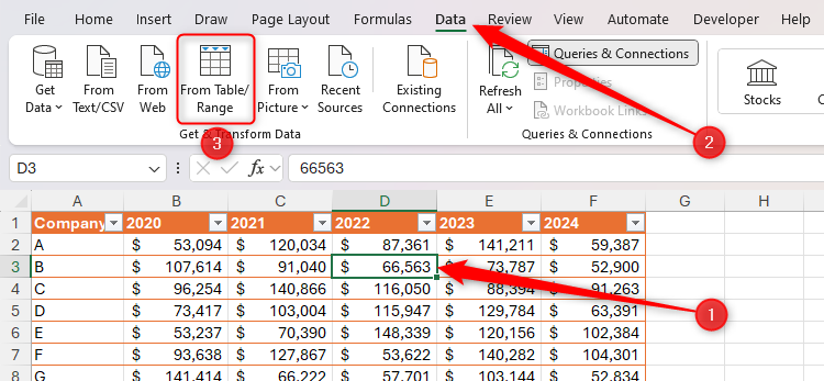
Compare the table in the example above to the following screenshot, where each column (field) contains identical data types.

As a result, it’s impossible to filter the data by year, and you can’t easily see which year was the most profitable for each company. To make these analyses, you’ll need to unpivot (or flatten) the data, which involves converting the data from a wide table into a long table by turning each year column into a row. In other words, you want all the financial values to be stored as a single field.

First, select any cell in the data, and in the Data tab on the ribbon, click “From Table/Range.”

At this point, if your data isn’t already formatted as an Excel table, you’ll see a dialog box prompting you to fix this. This is so that the Power Query Editor can read your data more easily.

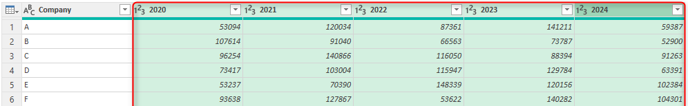
Then, in the Power Query Editor, select the headers of all the columns you want to unpivot. In this example, you’ll need to click the “2020” header, press Shift, and then click the “2024” header.

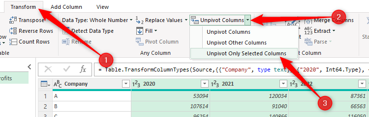
Now, in the Transform tab on the ribbon, expand the “Unpivot Columns” drop-down menu, and click “Unpivot Only Selected Columns.”

Now, each column is a separate field (company, year, and profit), and each row is a detailed company record.

Finally, double-click the column headers to rename them so that they match the field they represent, and click the number format icons to ensure each column contains the correct data type.

Now, when you click “Close And Load” in the Home tab on the ribbon, the unpivoted table is sent to a new spreadsheet in your Excel workbook.

As a result, you can perform data analyses that were impossible before you flattened the table, like filtering the data by year and company or sorting the company profits into descending order.

After adding more data to the original table, like another year of figures, head to the table produced previously by Power Query, and in the Query tab, click “Refresh.” Excel then adds the new data to the resultant table in its unpivoted format, saving you from having to return to the Power Query Editor each time.

4

Fill Blank Cells Based on the Cell Above (Or Below)

As I mentioned earlier, blank cells in a dataset can lead to issues when you sort and filter your data or use formulas that reference column headers, so it’s a good idea to fill them in.

In this example, only the first player in each team is assigned a team number in column A, so if you rearrange the data, you’ll lose sight of which player is in which team. Also, currently, you can’t filter the data by team number.

Ideally, cells A3 to A5 should contain the number 1, cells A7 to A9 should contain the number 2, and so on. Typing these numbers manually would be time-consuming, especially if, like in this example, there are many rows in the dataset. Instead, use Power Query to populate the blank cells in seconds.

First, with any cell in the data selected, in the Data tab on the ribbon, click “From Table/Range.”

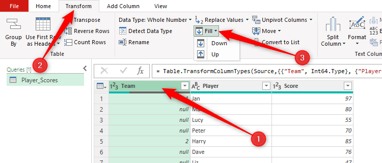
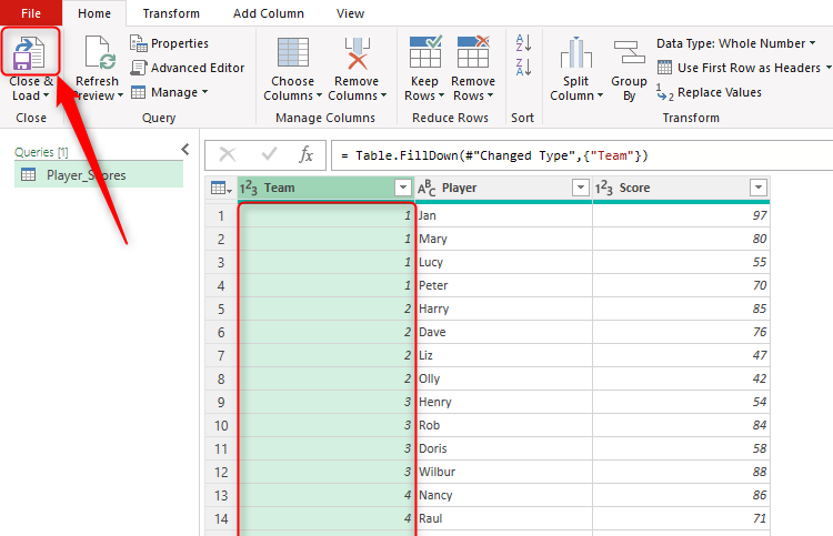
When the Power Query Editor opens, notice how the blank cells in the column in question contain the word “null.” To fix this, select the column by clicking the column header, and in the Transform tab, click “Fill.”

Then, choose whether you want to fill the data downward or upward. Clicking “Down” finds a cell in the selected range containing a value, and fills in any blank cells beneath with the same value. On the other hand, clicking “Up” fills blank cells above a cell containing a value. In this case, because only the first row of each team contains a number, you need to fill downwards.

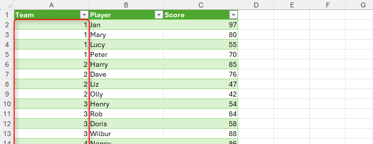
Now, each player is properly assigned a team number, so you can click “Close And Load” in the Home tab to send the query to a new worksheet.

Thanks to this quick but important change, you can sort and filter the dataset, safe in the knowledge that you won’t lose track of which player is in each team.

---

If you have multiple tables in separate Excel worksheets, providing they have the same column headers, you can use Power Query to stack the data into a single table. This involves the extra (but straightforward) step of creating data connections between each table, before combining the queries in the Power Query Editor.