How to Create a Drop-Down List from a Column of Data in Excel

Quick Links

Using a Column in a Formatted Excel Table

Using a Column in an Unformatted Dataset

Microsoft Excel’s Data Validation tool lets you add a drop-down list to a cell based on existing data in a column. However, how this works depends on whether the source data is part of a formatted Excel table. Let’s take a look at some examples.

Using a Column in a Formatted Excel Table

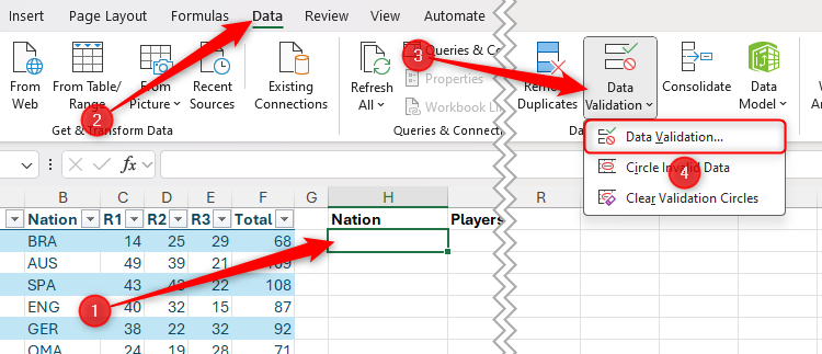
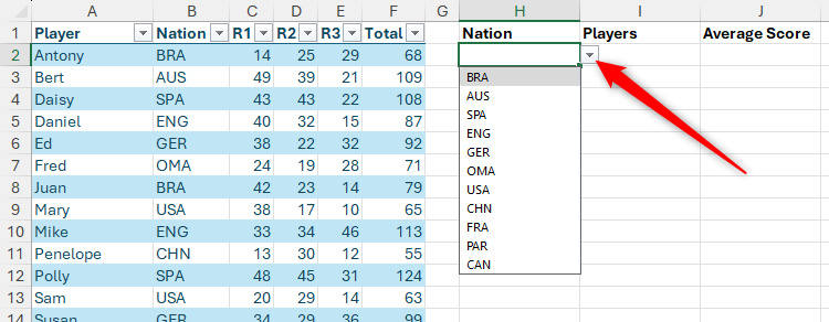
Imagine you have this formatted Excel table named “Scores” containing player names, nations, and scores, and you need to extract some summary data. Specifically, in cell H2, you want to create a drop-down list of all the nations listed in column B, and in cells I2 and J2, display the player names and average score, respectively, according to the nation selected.

To create a drop-down list, select cell where you want it to be (in this case, cell I2), and in the Data tab on the ribbon, click “Data Validation” in the drop-down option with the same name.

How to Add a Drop-Down List to a Cell in Excel

It beats typing in the same options 200 different times manually.

Then, in the Allow field of the Settings tab, select “List.”

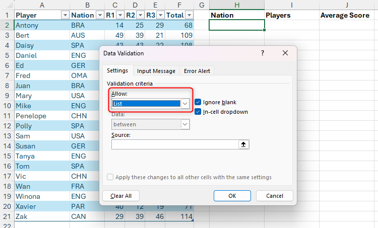
The next step involves inputting the options you want to appear in the drop-down list into the Source field. To do this, you can type the options manually, select the relevant cells on your spreadsheet, or use a formula.

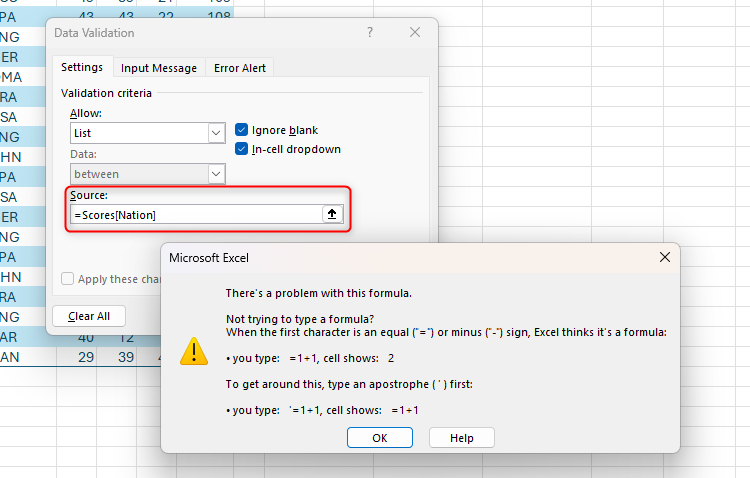
Ideally, you would be able to type:

=Scores[Nation]

into the Source field, exactly as you would when referencing that column in a formula, where “Scores” represents the table name, and “Nation” represents the column header. However, unfortunately, this returns an error message, as the data validation tool only recognizes cell references, formulas, and named ranges as data sources, not table column headers.

Luckily, there are two ways to get around this.

Method 1: Reference the Cells in the Table

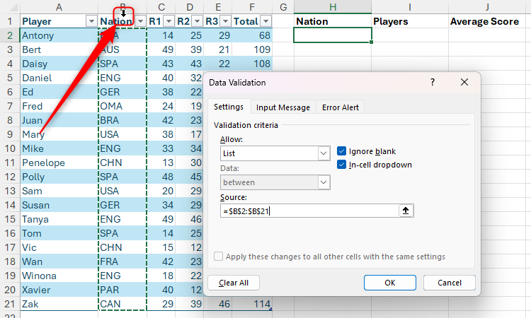
First, activate the “Source” field in the Data Validation dialog box so that the cursor is flashing, and hover over the relevant column header in row 1 until you see a small, black down arrow. When you do, click once to select all the data cells in that column.

Be careful not to select the whole column by clicking the arrow that appears when you hover over the column reference letter (in this case, “B”), as this will select the whole column, including the header in row 1 and the cells beneath your table. You’ve successfully selected the correct range if only the cells in the column within the table are surrounded by a dotted line.

Now, after clicking “OK,” when you select cell H2, a drop-down button appears, which you can click to select an option from the source. Notice, also, how only unique values are displayed in the list—in other words, Excel recognizes duplicate values, and only displays them once.

Data validation drop-down lists in Excel adopt the same order as the source. In this example, to order the nations alphabetically, you would need to sort the source data by column B.

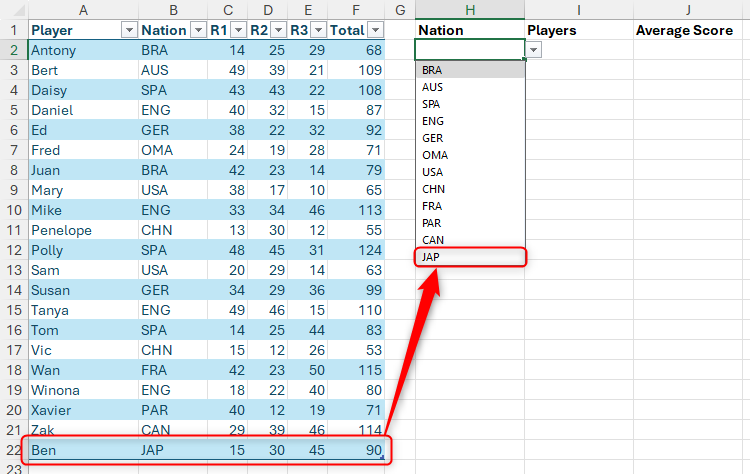
The beauty of using this method is that if you add more rows to the formatted Excel table, the data validation source automatically adjusts to include the extra cell or cells.

Now, you can use the FILTER function in cell I2 to list the selected nation’s players:

=FILTER(Scores[Player],Scores[Nation]=H2)

How to Use the FILTER Function in Microsoft Excel

There’s more than one way to filter your data.

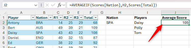
Finally, use the AVERAGEIF function in cell J2 to display the average score of players from this nation:

=AVERAGEIF(Scores[Nation],H2,Scores[Total])

How to Use the AVERAGEIF and AVERAGEIFS Functions in Excel

Be selective about what to include in your average calculations.

Method 2: Name the Range

The second way to create a drop-down list from a column in a formatted table involves naming the source range.

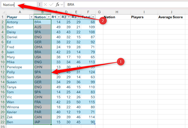
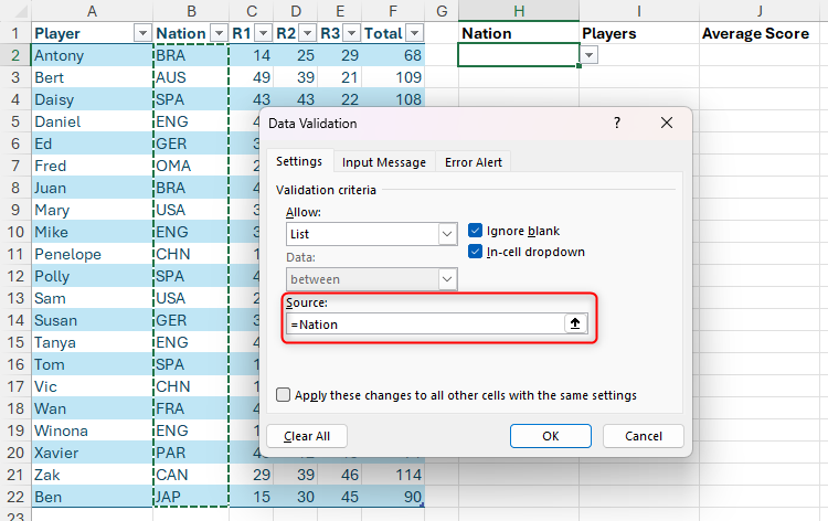
Before launching the Data Validation dialog box, select all the cells in the table that contain the values you want to include in the drop-down list, type a name for the range in the name box in the top-left corner of the Excel window, and press Enter.

To keep things simple (and memorable!), the name you enter for the selected range should be the same as the column header.

Then, in the Source field of the Data Validation dialog box, type an equal sign (=), followed by the name you just assigned to the range, and press Enter. In this example, you need to type:

=Nation

As with the previous method, Excel recognizes that the data is in a formatted table, so it automatically expands the range if data is added to the next row.

Using named ranges in Excel has many benefits. For example, naming ranges makes your workbook more accessible to people using screen readers. Also, you can quickly navigate to named ranges by typing them into the name box or selecting them from the options when you click the down arrow, and named ranges can also be used in formulas.

I Always Name Ranges in Excel, and You Should Too

Tidy up your Excel workbook.

Now, as with method 1, you can use the FILTER and AVERAGEIF functions to complete the data extraction.

However, this time, the formulas can be more straightforward, as you can reference the range you named “Nation” without referencing the table the range is in.

So, for FILTER in cell I2, it’s:

=FILTER(Scores[Player],Nation=H2)

and for AVERAGEIF in cell J2, it’s:

=AVERAGEIF(Nation,H2,Scores[Total])

Using a Column in an Unformatted Dataset

Certain types of data—like spilled arrays—cannot be formatted as an Excel table, so there may be times when you need to find a way to create a drop-down list from a column within an unformatted dataset.

After selecting the cell that will contain the drop-down list and clicking “Data Validation” in the Data tab on the ribbon, select “List” in the Allow field.

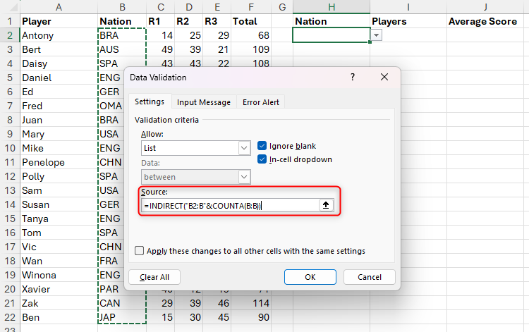
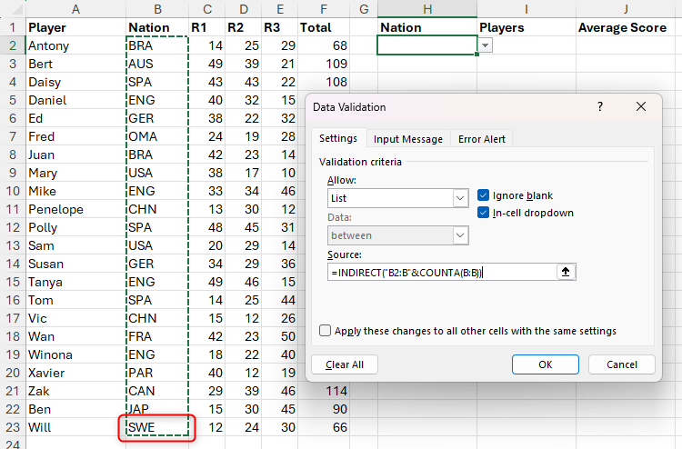
Next, in the Source field, use the INDIRECT and COUNTA functions together to tell Excel where to find the options for the drop-down list.

In this case, typing:

=INDIRECT("B2:B"&COUNTA(B:B))

includes all the values in column B from cell B2 to cell B22 as the source.

Let’s break this source formula down to see how it works.

=INDIRECT(: This tells Excel that you want the source to be determined using a dynamic reference.
“B2:B”: Specifically, the dynamic reference starts at cell B2, and ends at another cell in column B.
&COUNTA(B:B)): This counts all the cells in column B that aren’t blank, and adds the total to the reference. In this case, 22 cells in column B contain values, so this turns B2:B into B2:B22.

How to Use the INDIRECT Function in Excel

Use a text string to create a reference.

So, if you add another row of data at the bottom, the COUNTA function will pick this up and inform the INDIRECT reference in the data validation rule that the source has expanded downwards by an extra row.

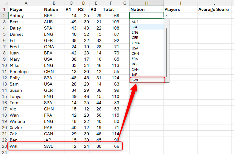
Using a formula to determine which values to include in the data validation source—rather than simply selecting the whole column—is considered best practice as it prevents the header row and blank rows from being included in the drop-down list.

You can double-check this by selecting the cell that hosts the drop-down list, and reopening the Data Validation dialog box. When you select the Source field, even though the formula hasn’t changed, the dotted line on the spreadsheet confirms that it picks up the new values in the added row.

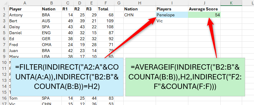
Now that your drop-down list is ready to go, use the INDIRECT and COUNTA functions alongside the FILTER function in cell I2 and the AVERAGEIF function in cell J2 to complete the spreadsheet.

Drop-down lists added through the Data Validation tool are incredibly powerful and versatile, and can be used in many scenarios in Excel. For example, you can use drop-down lists to make regular charts dynamic—a surefire way to impress your friends and coworkers.

Source link