How-To Geek’s A to Z of Key Microsoft Excel Jargon

Do you know the difference between an array and a range? How about differentiating between a function and a formula? Excel has hundreds of key terms, and some are more intuitive than others. Understanding some of the jargon will go a long way to helping you understand other aspects of the program.

Microsoft has its own Excel glossary containing hundreds of terms and definitions. However, in this article, we have chosen some of the more frequently used terms that will get you on your way, whether you’re reading an Excel How-To Geek guide or you’ve applied for a job that requires Excel knowledge. In short, this is a must-know list, not a comprehensive list.

A

Active: An Excel worksheet, its content, or a cell is active when selected. The name of the active worksheet will appear as a bold tab at the bottom of your window, and the active cell will have a bold border.

Add-in: Tools that you install on your computer to create additional functions in Excel, such as a translation or a calendar add-in.

Array: A set of data within a range of cells. For example, if cells A1 to A20 contain data, A1:A20 is the range, and the data within those cells is the array. An array formula is used to perform multiple calculations at the same time.

B

Border: A line that is added to the outside of a cell or object. Cells can have top, bottom, left, or right borders, or a combination of any of these. While gridlines do not print by default, borders do.

C

Cell (reference): A cell is an Excel box that is distinguished by the gridlines, and each cell edge is a row or column line. Each cell contains its own data and has its own reference. A cell reference is its column and row location (for example, cell B2 is in column B, row 2).

Conditional Format: Formatting that is automatically applied to a cell based on specific conditions. For example, all cells containing the word “DONE” might have a green background due to conditional formatting rules that have been applied to those cells. Excel offers preset conditional formatting rules, or you can define specific parameters. Click Home > Conditional Formatting.

Criteria: Also known as conditions, criteria determine which cells are filtered, evaluated, or counted. For example, an Excel formula containing the COUNTIF function will count the cells containing certain criteria.

D

Data Validation: When applied (via Data > Data Validation), data validation limits what can be entered into a cell. For example, you can define a cell to contain only whole numbers or dates. You can create an error message that appears when the wrong type of data is inserted into a cell, and you can also add a message that appears when a user clicks the cell containing the rule. Data validation can also be used to create a drop-down list of options to appear in the cell.

Drop-down: A list of choices that appears when a trigger is clicked. For example, a drop-down list can appear when you click an option on the ribbon, a filter button in a cell, or a cell containing data validation rules.

E

Embed: You can embed a snippet of another file into an Excel worksheet (via Insert > Object). You can also embed a chart within a worksheet, rather than creating a new Excel chart sheet.

F

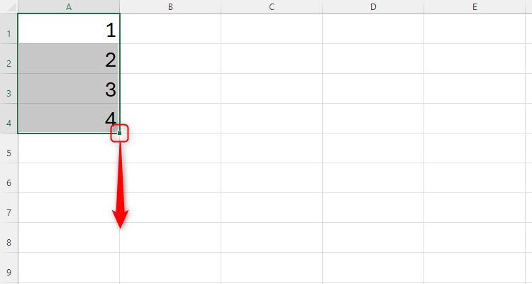
Fill handle: The small, black dot in the bottom-right corner of a cell, which you can click and drag to apply the same formula to other cells in a range. You can also use the fill handle to make Excel continue a sequence that you have begun across a range of cells.

Filter: Filters let you display only the values in a column that meet the conditions you set. You can also use the FILTER function to filter data by multiple criteria.

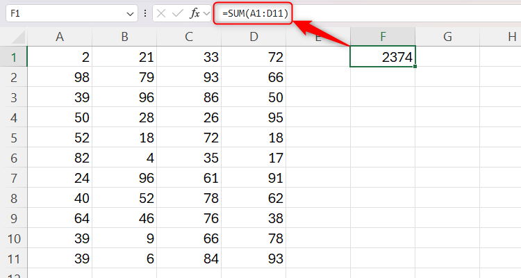
Formula (bar): A formula is a combination of functions, cell references, values, operators, and names that, when used together following the equals (=) sign, create a new value. For example, =SUM(A1:D11) is a formula that adds the values in cells A1 to D11, and produces the outcome in the cell where the formula is entered. While the outcome appears in the cell, the related formula appears in the formula bar at the top of the Excel window, where you can edit the formula.

Function: A pre-defined formula that performs a calculation when used in a formula. For example, the AVERAGE function finds the mean of the referenced values or cells.

G

Gridlines: Non-printing lines that represent boundaries between cells. You can also add gridlines to charts to make reading the data easier.

H

History: You can view an Excel workbook’s version history to see the changes that have been made, or revert to a previous version.

L

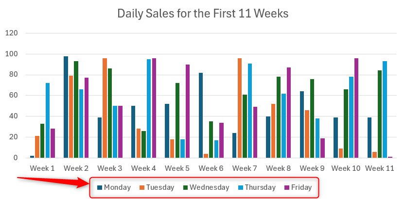
Legend: In a chart, a legend tells the viewer what each color or pattern refers to. For example, different colors could represent different days in a chart, and the legend makes this clear.

M

Merge: Merging adjacent cells removes their separating gridlines and combines them structurally to create a larger cell.

N

Name (box): A name is a word or combination of words that represent a cell reference, table, or formula. A name can be used in a formula to avoid having to reference an individual cell or range of cells. The name box, situated to the left of the formula bar at the top of the Excel window, displays the names used in a workbook and can be used to quickly jump to a named item.

O

Operator: A symbol that identifies and dictates a calculation to be performed. These include arithmetic operators (such as + and -), logical operators (such as AND and OR), comparison operators (such as = and >), and more.

P

Pivot Tables and Pivot Charts: Pivot tables and charts let you visualize data in a bespoke way, meaning you can summarize data and identify patterns quickly.

Power Query: A tool that lets you import and shape data from different sources, and then load the data onto a worksheet.

Protect: Protecting a workbook or a worksheet means you can prevent others from performing certain actions—such as selecting certain cells, changing the formatting, and others—by adding a password.

R

Range: Two or more cells on a worksheet. Cells in a range can be adjacent (contiguous) or non-adjacent (non-contiguous).

S

Series: An array of data in a range that is entered into a chart to be visualized graphically.

Sort: You can rearrange data in a column or table based on value, formatting, or conditional formatting.

T

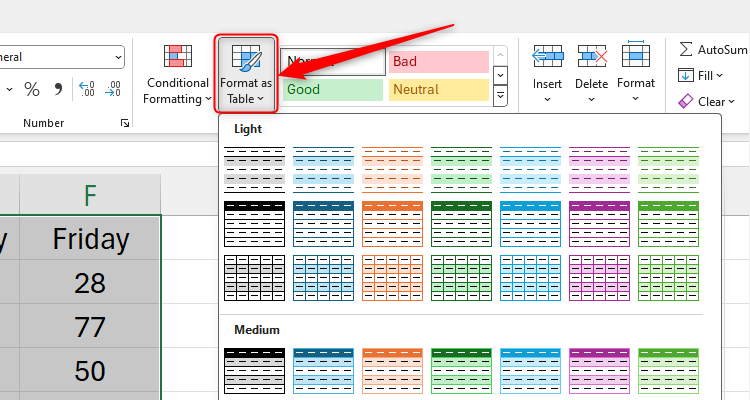
Table: Formatting data as a table via the Home tab means that all the rows and columns are linked together, the range can be named for use in formulas, and more data can be easily added.

V

View: There are four different workbook views. The Normal view is the default view in which you do most of your Excel work, the Page Break view shows you where the page boundaries will be when you print your worksheet, the Page Layout view is where you can see the page measurements and add headers and footers, and the Custom Views allow you to define what you see on your screen when using Excel.

W

Workbook: An Excel file containing one or more worksheets.

Worksheet: An individual spreadsheet within a workbook where data is added. A single workbook can have multiple worksheets that are created, removed, named, and ordered via the tabs at the bottom of the workbook window.

Now that you’ve picked up some essential Excel jargon, check out the most useful Excel keyboard shortcuts that will help you work much more efficiently.