Global subsidence of river deltas

Selection of global river deltas

We selected 40 deltas globally, prioritizing 35 deltaic systems with the greatest exposed area and population currently below sea level, supplemented by five less-exposed deltas of local and regional significance and previously identified risks⁹. To assess the 35 deltas with the greatest exposure among global river deltas, we used 955 delineated delta boundaries in ref. ⁶ and identified coastal delta elevation below sea level using the DeltaDTM dataset v.1.1 (ref. ¹¹) resampled to 3 arcseconds (100 m) and referenced to mean sea level⁵¹. Global delta population was estimated by aggregating 100 m resolution WorldPop population count for each delta, which is calibrated to the 2020 national population estimates from the United Nations population data⁵².

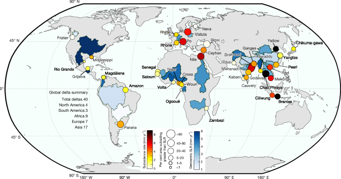
Our estimates show that globally, 42,000 km² of the delta area at present lies below sea level, containing a population of 10.2 million people (Extended Data Fig. 1). The 35 deltas with the greatest exposure included in this analysis are Nile, Mississippi, Rhine–Meuse, Mekong, Niger, Cauvery, Po, Red River, Vistula, Rhone, Amazon, Ganges–Brahmaputra, Chao Phraya, Kabani, Pearl, Rio Grande, Yangtze, Yellow River, Senegal, Indus, Saloum, Grijalva, Ceyhan/Seyhan, Rioni, Cross, Chikuma-gawa, Volta, Brantas, Neva, Wouri, Irrawaddy, Ogooué, Zambezi, Magdalena and Ciliwung (Extended Data Fig. 1). The cumulative delta area and population below sea level are 38,000 km² and 10.1 million people, respectively, reaching within rounding errors of the global total exposure. Deltas such as the Danube, Orinoco and Shatt-el-Arab met the selection criteria but were excluded due to challenges associated with the SAR imaging and interferometric analysis (including spatial coverage gaps, excessive temporal baselines, poor coherence and limited data availability). The five supplementary deltas are Brahmani, Mahanadi, Godavari, Parana and Fraser deltas.

The final selection of 40 deltas spans five continents (Asia, Africa, Europe, North America and South America) and 29 countries, encompassing deltas with noted and emerging environmental, geophysical and social vulnerabilities^9,24, historically sinking river deltas² and densely populated coastal megacities^3,4,53.

SAR dataset

We analysed 132 SAR frames from the Sentinel-1A/B C-band satellite, spanning September 2016 to May 2023. The SAR datasets include 3,300 images obtained in single-orbit geometry (ascending or descending) for 13 deltas and 10,700 images obtained in both ascending and descending orbits for 27 deltas. See Supplementary Table 3 for the complete inventory of SAR images used in each delta. For each SAR dataset, we applied a multi-looking factor of 32:6 (range:azimuth) to improve the signal-to-noise ratio, obtaining an average pixel resolution of about 75 m. To minimize decorrelation errors, we also constrained the interferometric pairs to a maximum temporal and perpendicular baselines of 300 days and 80 m, respectively. For deltas requiring multi-frame coverage (for example, Amazon, Mississippi, Mekong, Ganges–Brahmaputra, Nile, Red River and Niger), we arranged in a mosaic form the overlapping adjacent frames along a single path before processing or post-processed deltas with coverage spanning multiple paths to ensure full spatial continuity across expansive deltas.

SAR interferometric analysis

We processed each SAR frame or single-path multiple-frame coverage to generate high-spatial resolution maps of surface deformation for the 40 deltas using a multitemporal wavelet-based InSAR (WabInSAR) algorithm^54,55,56,57. First, we generated 59,000 high-quality interferograms from the coregistered SAR images using GAMMA software^58,59, with an interferogram pair selection algorithm⁵⁷ optimized through dyadic downsampling and Delaunay triangulation. To minimize phase errors and to maximize the pixel density associated with dynamic surface changes over deltas (for example, flooding, vegetation growth or soil saturation), we screened the initial set of interferograms based on their coherence stability to exclude interferograms with high coherence variability, while maintaining a 50% temporal baseline coverage. The final selection retained about 55,000 interferometric pairs (93%) for further analysis. Moreover, we implemented a statistical framework to discard noisy pixels with average coherence less than 0.7 for distributed scatterers and amplitude dispersion of greater than 0.35 for permanent scatterers⁵⁷. Next, we used a minimum cost flow phase unwrapping algorithm optimized for sparse coherent pixels^60,61 to estimate the absolute phase changes of the elite (less noisy) pixels in each interferogram. We corrected all unwrapped interferograms for the effects of residual orbital error⁶² and minimized the effects of topography-correlated components of atmospheric phase delay and spatially uncorrelated DEM error by applying a suite of wavelet-based filters⁵⁴. Last, we estimated the time series, velocities and standard deviation for each geocoded elite pixel along the line of sight (LOS) of the satellite using a reweighted least-squares optimization⁵⁵. The standard deviation of the LOS velocity corresponds to the uncertainty of the regression slope derived from the least-squares fit. For each delta, the reference point was selected as the pixel corresponding to a global navigation satellite systems (GNSS) station within the processed SAR frame when available. In areas without GNSS stations, a preliminary reference point was randomly selected from pixels with average temporal coherence >0.85. Following initial processing, the reference point was refined by visually identifying stable ground features (for example, bedrock outcrops and deep-foundation structures) and low displacement variability (standard deviation <1 mm yr^–1), then reprocessing with this final reference point. For large deltas requiring overlapping SAR frame coverage, the LOS velocities were arranged in a mosaic form to ensure seamless spatial representation across the entire delta.

In the 27 deltas with overlapping spatiotemporal SAR satellite coverage and different orbit geometries (ascending and descending), we estimate the horizontal (east–west) and VLM components of deformation by jointly inverting the LOS time series of the ascending and descending tracks^63,64,65. To this end, we identified the co-located pixels of the LOS time series by resampling the pixels from the descending track onto the ascending track to obtain two co-located LOS displacement velocities \(\{{\mathrm{LOS}}_{\mathrm{ASC}},{\mathrm{LOS}}_{\mathrm{DES}}\}\). Given \(\{{\mathrm{LOS}}_{\mathrm{ASC}},\,{\mathrm{LOS}}_{\mathrm{DES}}\}\) and their associated variances \(\{{\sigma }_{\mathrm{ASC}}^{2},{\sigma }_{\mathrm{DES}}^{2}\}\) are the LOS displacement and variances for a given pixel, the model to combine the LOS velocities to generate a high-resolution map of the east–west (E) and VLM (U) displacements are given by

where, C represents the unit vectors for projecting (E) and (U) displacements onto the LOS, which is a function of the heading angle of the satellite and incidence angles of each pixel⁶⁶. The solution to the model in equation (1) is given by

where X represents the unknowns (E) and (U), G is the design matrix comprising the unit vectors for projecting the horizontal and vertical displacements onto the line of sight, L are the observations \(\{{\mathrm{LOS}}_{\mathrm{ASC}},{\mathrm{LOS}}_{\mathrm{DES}}\}\), and P is the weight matrix, which is inversely proportional to the observant variances \(\{{\sigma }_{\mathrm{ASC}}^{2},{\sigma }_{\mathrm{DES}}^{2}\}\). To obtain the parameter variance–covariance matrix (Q_XX), we use the concept of error propagation⁶⁷ to calculate the associated parameter uncertainties given the observation errors as follows:

For the 13 deltas imaged in single-orbit geometry (ascending or descending), we projected the LOS velocities to the vertical direction, assuming the principal deformation is vertical:

where, cosθ_i is the local incidence angle for each pixel. This assumption of zero gradients in the horizontal components of deformation is tenuous for most coastal areas, given the significant localized horizontal motion noted (up to 10 mm yr^–1) across the 27 deltas with multiple orbit geometries. Nevertheless, the assumption is necessary given that overlapping ascending and descending orbit geometries are available for less than 50% of global land areas (for European Space Agency Sentinel-1 satellite), limiting the ability to resolve 2D deformation trends. However, under this assumption, it is necessary for the locally referenced VLM estimates to be transformed into a globally consistent reference frame, particularly for comparative studies across multiple regions^13,27.

To transform the VLM rates from a local to a global reference frame, we used the available GNSS datasets for 17 deltas (the Fraser, Mississippi, Rio Grande, Rhine–Meuse, Rhone, Po, Vistula, Red River, Amazon, Parana, Ciliwung, Brantas, Ganges–Brahmaputra, Chao Phraya, Mekong, Pearl and Chikuma-gawa). The GNSS datasets across the 17 deltas were obtained from the Nevada Geodetic Laboratory⁶⁸ and previous regional studies⁶⁹. For each delta with GNSS coverage, we calculated the offset between the InSAR-derived vertical velocity at the reference point and the corresponding GNSS vertical velocity, then applied this offset to transform all InSAR velocities in that delta to the IGS14 reference frame. The uncertainty in the final velocity was estimated by propagating both the InSAR velocity uncertainty (from the reweighted least-squares inversion) and the GNSS velocity uncertainty (reported by data sources) through standard error propagation. In deltas without GNSS stations, we used the global VLM model⁷⁰, which mainly includes long-wavelength deformation signals due to TWS changes, tectonics and glacial isostatic adjustment (GIA) referenced to the IGS14 global frame. We then applied an affine transformation to align the VLM rates from local to IGS14 global reference frame^23,71. This approach ensures consistency in VLM rates across global deltas by correcting for local reference biases and should be the standard practice in coastal research using InSAR²⁷. When comparing these measurements to other subsidence rate estimation techniques in deltas, such as RSET, marker horizons, sediment cores, repeat lidar or other InSAR measurements, careful consideration must be given to differences in both reference frames and temporal ranges. Reference frame incompatibility may require adjustments to align local or relative measurements with other datasets, whereas mismatches in monitoring periods introduce temporal biases that complicate direct quantitative comparisons.

The distribution of the standard deviations (precision of the results) for all pixels (20.5 million) across the 40 deltas is shown in Supplementary Fig. 2. The standard deviation distribution shows that 99% of the pixels have a value <0.5 mm yr^–1. We evaluated the accuracy of the results by comparing the averaged VLM rates of pixels within a radius of 100 m with more than 100 independent GNSS data (that is, stations that were not used in the reference frame transformation). The validation included 122 GNSS stations across 23 deltas with historical long-term records (spanning various periods before and/or including the InSAR observation window) and 81 GNSS stations across 15 deltas with time series covering at least 70% of the InSAR observation period (2014–2023) (Supplementary Fig. 3). We found a strong correlation (0.7–0.8), between GNSS and InSAR velocities, with an RMSE of 1.4 mm yr^–1 for long-term rates (Supplementary Fig. 3a) and 1.2 mm yr^–1 for rates within the InSAR observation period (Supplementary Fig. 3b). The improved agreement for temporally coincident measurements suggests that nonlinear subsidence behaviour contributes to some scatter when comparing historical GNSS rates to contemporary InSAR measurements, although the overall correlation remains strong in both cases. Note that some GNSS stations used for validation, while within the broader processed SAR frame, are outside the clipped delta boundaries. Note that the final delta extents were delineated using a tiered approach. Primary boundaries were derived from ref. ⁹, supplemented by ref. ⁶ for deltas not covered in the former. For extensive deltas in which the entire delta surface is not analysed (for example, the Ganges–Brahmaputra), boundaries were defined using the SAR spatial extent.

GIA influence on VLM

We estimated VLM trends and the associated uncertainty due to GIA using the model in ref. ⁷², which was derived from a probabilistic ensemble of 128,000 GIA forward simulations. Each model solves the sea-level equation for a compressible, viscoelastic Maxwell Earth under late-Pleistocene ice-sheet loading, incorporating solid-Earth deformation, geoid change and rotational feedback. The ensemble samples a wide range of Earth rheological structures, including lithospheric thickness, upper and lower mantle viscosities, and scaling factors applied to regional deglaciation histories over the past 122,000 years. Likelihoods were assigned to each simulation based on fit to a global dataset of 11,451 relative sea-level records and 459 GNSS-derived uplift rates using a Bayesian framework that accounts for data uncertainties and spatial correlations. The resulting posterior distributions enable spatially resolved estimates of GIA-driven VLM with formal uncertainty.

For each delta, we extracted the ensemble mean and standard deviation in GIA vertical velocity to correct observed deformation rates and isolate contemporary, non-GIA contributions to VLM. Supplementary Table 1 shows the mean GIA-induced VLM, the associated standard deviation and the per cent contribution of GIA to the total observed VLM magnitude for each delta. GIA accounts for the largest proportion and exceeds (>100%) the total VLM in the Neva (540%) and Fraser (455%) deltas, in which low observed VLM rates are substantially influenced by strong GIA uplift. Moderate GIA contributions (25–55%) are observed in five deltas, including the Rio Grande, Mississippi, Volta, Rhine and Ogooué deltas. Most of the deltas (55%) exhibit minimal GIA influence, with contributions under 10%, indicating that observed VLM is primarily governed by contemporary anthropogenic and natural processes such as groundwater withdrawal, sediment compaction, or tectonics. In 28–67% (accounting for uncertainty) of the deltas, the sign and approximate magnitude of observed and GIA-corrected VLM are consistent, implying limited distortion from GIA and the sustained expression of contemporary processes on the average local subsidence. By contrast, the Fraser and Neva deltas illustrate how substantial GIA-induced uplift in high-latitude, post-glacial regions can obscure contemporary subsidence processes through opposing vertical trends. In both cases, modest observed subsidence rates (Fraser −0.4 mm yr⁻¹ and Neva −0.2 mm yr^–1) are counteracted by substantial GIA uplift of 1.8 ± 2.3 mm yr⁻¹ and 1.0 ± 0.3 mm yr⁻¹, respectively.

Anthropogenic drivers datasets

We analysed the relationship between major anthropogenic pressures on global deltas to subsidence and elevation loss by quantifying the contributions of groundwater storage change, sediment flux alteration and urban expansion to the residual rates of sinking (after GIA correction) across the 40 deltas. These globally consistent datasets provide insights into human-induced impacts on land subsidence and elevation change in river deltas (Supplementary Table 2).

Groundwater storage change

We derived twenty-first-century groundwater storage trends for all deltas by leveraging Gravity Recovery and Climate Experiment (GRACE) and GRACE Follow-On (GRACE-FO) satellite observations^73,74. We used the JPL GRACE/GRACE-FO level 3 mascon solutions (RL06.3) (refs. ^75,76), which provide monthly global estimates of total water storage (TWS) change relative to a 2004.9–2009.999 mean baseline. The final solutions span 2002–present and are derived from solving for monthly gravity field variations in terms of 4,551 equal-area 3° spherical cap mass concentration functions rather than global spherical harmonic coefficients. The mascon approach implements geophysical constraints during the level-2 processing step to filter out noise, applies improved accelerometer data and standard corrections, including several geophysical adjustments, such as gravity anomaly due to ocean (GAD), GIA, degree-1, C20 and C30 replacement and representation on ellipsoidal earth^75,76,77. We extracted TWS values at 3° mascon resolution (about 300–400 km spatial resolution) covering each delta area to compute representative regional water storage estimates. TWS change from GRACE contains contributions from GWS, soil moisture storage (SMS), snow water equivalent (SWE) and surface water storage (SWS) represented by

To isolate GWS change from TWS, we used the 1/4° global land data assimilation system Noah model⁷⁸ to remove changes in SMS and SWE contributions and used the WaterGAP Global Hydrology Model (WGHM v.2.2d) (refs. ^79,80) to remove SWS contributions. The contribution from SWE was negligible in most deltas, given their prevailing arid and semi-arid climate (Fig. 1), although it was included to maintain consistency across all deltas. SWS components include contributions from rivers, lakes, wetlands and reservoir storage within the GRACE footprint for each delta. The residual signal following removal of SWS, SMS and SWE was interpreted as the GWS anomaly.

To estimate the temporal trend of groundwater storage changes, we applied harmonic analysis to account for annual and semiannual variations in the time series of the GWS anomalies. In standard practice, environmental variables (for example, GRACE data, GNSS data and sea-level anomalies) are modelled as time-invariant seasonal signals. However, the response of Earth to environmental changes represented as seasonal signals is not time-invariant^81,82,83. To account for this variability, we adopted the stochastic-seasonal model in the following equation, in which the harmonic amplitudes evolve as random walks, allowing for time-dependent seasonal variations and the seasonal trends are modelled using a Kalman filter⁸³:

where t₀ is the reference epoch, x₀ is the reference intercept at t₀, v(t) is the time-varying rates, k indexes the annual (k = 1) and semiannual (k = 2) components, a_k and b_k are the harmonic amplitudes. v(t), a_k, and b_k are modelled as random walk parameters. To estimate the long-term multi-year trend (v_f) of GWS from the time-varying rates, we computed the weighted average of the time-varying rates v(t_i) using

where m is the total number of epochs in the time series and \({\sigma }_{v({t}_{i})}^{2}\) is the variance of the rate at epoch t_i, derived from the posterior covariance matrix of the Kalman filter. The uncertainty \({\sigma }_{v}^{2}\) in the rate is given by

Supplementary Figs. 4 and 5 compare the time-invariant model (black curves) with the stochastic-seasonal model (red curves) for GRACE-derived GWS and RSLR from tide gauges in the Mississippi and Chao Phraya deltas. These plots show that a stochastic-seasonal process better represents the observed variability in the time series. The post-fit residuals of the time-invariant model show some systematic seasonal patterns, particularly during periods when seasonal amplitudes deviate from the assumed constant values (Supplementary Figs. 4b,d and 5b,d). By contrast, the stochastic model accommodates time-dependent variations in seasonal amplitudes, resulting in reduced (often near-zero) residuals (Supplementary Figs. 4b,d and 5b,d), demonstrating the advantage of the stochastic-seasonal model in capturing transient seasonal variations rather than fixed annual and semiannual cycles⁸³.

The GWS rates for each delta are summarized in Supplementary Table 2, and Fig. 3a and Extended Data Fig. 8a show the relationship with the subsidence rates. Negative GWS trends indicate mass depletion, primarily driven by groundwater extraction, whereas positive trends represent net groundwater accumulation due to recharge processes, reduced extraction or hydrological interventions. To evaluate the reliability of GRACE-derived GWS trends, we compared them with in situ groundwater level trends for 18 deltas (Supplementary Fig. 6). Groundwater levels were compiled from two publicly available sources: 13 deltas from ref. ⁸⁴ and 5 deltas from the Global Groundwater Monitoring Network⁸⁵. Given the spatial scale discrepancy between GRACE (basin-wide) and well observations (point-scale), we emphasized agreement in trend direction rather than absolute magnitudes. Each site was categorized based on the sign of the GRACE and well trends, and a confusion matrix was constructed to assess consistency. The analysis yielded an overall classification accuracy of 88.9%, with six sites exhibiting positive–positive trends (PPT) and 10 showing negative–negative trends (NNT). Only two sites showed mixed behaviour (NPT or PNT), and no site exhibited fully opposing trends. Moreover, a high correlation (R = 0.7) was observed between the GRACE-based GWS and well-derived trends, further supporting the consistency of GRACE estimates at the basin scale despite localized variability in in situ measurements. Although the coarse spatial resolution of GRACE/GRACE-FO may not capture localized variations⁸⁴, its basin-scale sensitivity is well-suited to characterizing basin-wide groundwater trends. Moreover, the dominance of groundwater extraction in many deltas^2,20,31 probably ensures that GWS trends are the primary signal captured.

We find a modest linear correlation (R = 0.5) between GWS and subsidence rate; however, a cubic regression model (R = 0.6) provides a better fit (Extended Data Fig. 8a).

Sediment flux alteration

We obtained values for the sediment flux alteration for the 40 deltas from ref. ²⁹. This dataset provides a global assessment of fluvial sediment supply, distinguishing between pristine sediment fluxes (before substantial anthropogenic influences) and disturbed or contemporary sediment fluxes (reflecting human influences such as dam construction and land-use changes) within the contributing delta basins. We quantified the per cent change in sediment flux for each delta using the following equation, which expresses the relative alteration (increase or decrease) in sediment delivery due to human activities:

The pristine and disturbed sediment flux, along with computed sediment flux changes for each delta, are summarized in Supplementary Table 2. A negative sediment flux change indicates a decline or loss in fluvial sediment supply (disturbed < pristine) due to human activities, whereas a positive sediment flux change reflects an increase or gain (disturbed > pristine). We acknowledge that this framework represents a simplified characterization of complex sediment delivery processes and may not capture all temporal variations in sediment supply. Furthermore, some concerns have been raised about potential errors in global sediment flux datasets⁸⁶, which we consider as a limitation in our analysis.

Figure 3a and Extended Data Fig. 8b show the relationship between sediment flux change and subsidence rates. Although a poor correlation (R < 0.4) is observed, we find that 62% of the deltas (25 out of 40) exhibit negative sediment flux change, indicating widespread human-induced reductions in sediment supply.

Urban expansion

Urban expansion is one of the most visible and rapid types of ongoing anthropogenic changes in river deltas⁶. To assess how population-driven land-use changes may affect subsidence rates across deltas, we used a global 1/8° (about 12.5 km) urban land fraction dataset, derived from high-spatial-resolution remote sensing observations⁸⁷. This dataset tracks the conversion of natural landscapes (that is, wetlands and forests) into built environments and serves as a proxy for land-use changes that may exacerbate subsidence through increased infrastructure loading and increased groundwater demand. We quantified the urban fraction change in deltas in the twenty-first century by calculating the percentage change in the proportion of urban areas relative to total delta area between 2000 and 2020.

Supplementary Table 2 summarizes the urban fraction dataset (2000 and 2020) and the urban fraction change for each delta. Figure 3a and Extended Data Fig. 8c show the subsidence–urban expansion relationship across the 40 deltas. All deltas showed consistent urban expansion in the twenty-first century, ranging from relatively low increases (<1%) in the Ogooué river delta to significant increases (>400%) in the Indus delta. However, despite this rapid expansion, the Indus delta remains one of the least urbanized, with only 0.4% of its total area classified as urban in 2020. By contrast, the Ciliwung (Jakarta) and Neva (Saint Petersburg) deltas exhibit the highest urban fractions, exceeding 50%. A logarithmic fit best describes the full dataset and reveals a moderate but significant nonlinear inverse correlation (correlation, R = 0.38–0.51), indicating that deltas with significant urban land conversion tend to experience more pronounced land sinking (Extended Data Fig. 8c). Steadily urbanizing deltas, such as the Rio Grande and Rhine–Meuse, exhibit slower subsidence rates, whereas rapidly urbanizing deltas, such as the Brahmani and Yellow River deltas, show faster rates of land sinking. However, regional variability is evident, as some deltas deviate from the overall trend (for example, Indus and Cauvery deltas). When excluding outliers (the Indus and Cauvery deltas), subsidence and urban expansion exhibit a strong linear correlation across deltas (Extended Data Fig. 8c).

We also explored the relationship among the anthropogenic drivers (Extended Data Fig. 8d–f), finding a low (R = 0.1–0.3) correlation depending on the specific driver.

RF analysis for identifying anthropogenic drivers of subsidence and elevation loss

Given the nonlinear and interacting relationships among GWS, sediment flux alteration, urban expansion and residual land subsidence (after GIA correction) discussed above, a machine learning framework was implemented to model these complexities. First, we attempted a multilinear regression model, incorporating interaction terms between variables, formulated as

where VLM is the predicted VLM, x₀ is the intercept, X_i,j,k are the predictor variables (GWS, sediment flux alteration and urban expansion), x_i,j,k are the regression coefficients for each predictor variable, x_jk represents the interaction effects between predictor variables and ϵ is the residual error term. However, this multilinear regression model yielded poor performance (correlation R = 0.38; R² = 0.15; RMSE = 4.7 mm yr¹) (Fig. 3a), demonstrating the inefficiency of linear models to capture these complex dependencies and the need for a machine learning model.

Next, we used an RF machine learning model to better account for these complex nonlinear interactions between variables. RF has been widely applied in environmental and hydrological studies to model complex systems with nonlinear dependencies, outperforming traditional regression techniques in similar contexts^{88,89,90,91,92}. The RF model is well-suited for this analysis due to its ability to handle small datasets (40 deltas), its simpler hyperparameter tuning, and its ability to compute feature importance. In this study, the primary objective for applying RF is not to predict the subsidence rates, but rather to extract key features that explain the dynamic relationships between anthropogenic drivers and subsidence across global deltas.

The RF algorithm is an ensemble learning method that uses the strength of multiple independent regressor decision trees {T}, in which each tree {T_t} is trained on a randomly sampled subset of the input features ({X = X₁, X₂, X₃}, representing GWS, sediment flux and urban expansion) through bootstrap aggregation (bagging). Key hyperparameters, including the number of trees, maximum tree depth, minimum samples per split and minimum samples per leaf, were optimized using grid search with five-fold cross-validation to minimize overfitting and maximize predictive accuracy⁹³. This ensemble approach enhances predictive performance by creating a learning environment in which a large number of predictors work on various characteristics of the input features and learn to combat overfitting and generate predictions (VLM) by computing the average of all decision tree predictions:

The RF regressor optimizes each decision tree using the mean square error (MSE) defined as a cost function to identify node splits and model performance during model training and testing:

where VLM_i is the observed VLM rate for individual delta i, \(\hat{{{\rm{V}}{\rm{L}}{\rm{M}}}_{{i}}}\) is the predicted VLM rate and N is the total number of observations. To assess uncertainty, we used Monte Carlo simulations to create multiple holdout fractions (0.1–0.5) across 100 iterations, randomly subsampling the 40 deltas for training and validation in each iteration. This random partitioning ensures that each delta is used in both training and validation phases across iterations, enhancing the robustness against overfitting and sampling bias. The final RF model predictions were obtained by averaging prediction estimates across all iterations. The final model performance was evaluated using the coefficient of determination (R²), RMSE and mean absolute error (MAE):

where \(\bar{{{\rm{V}}{\rm{L}}{\rm{M}}}_{i}}\) is the mean observed VLM rate, and the other variables are defined in equation (12). The feature importance I_f for input feature {X = X₁, X₂, X₃} was computed using the following equation, based on the cumulative reduction in node, j impurity among all the trees:

where N denotes the total number of trees and ΔI_j denotes the change in impurity.

Although RF effectively captures nonlinear relationships, its ensemble structure limits delta-specific interpretability. To resolve local insights into delta-specific subsidence drivers, we applied LIME, a technique within the field of explainable artificial intelligence (XAI)⁹⁴. LIME approximates black-box models such as RF by fitting interpretable models to perturbed samples of the input data, allowing for local feature importance estimation. For each delta X_i, LIME approximates the RF prediction locally by using a linear surrogate model trained on perturbed instances around X_i. The explanation function is obtained by solving the following minimization problem:

where ξ(X_i) is the local interpretable model for each delta X_i, g is the interpretable model, f is the RF model, \({{\rm{\pi }}}_{{X}_{i}}\) is a proximity kernel, \(L(f\,,g,{{\rm{\pi }}}_{{X}_{i}})\) is the loss function measuring the differences between f and g, and Ω(g) penalizes complexity. This process was repeated for each delta, and deltas with low LIME model fidelity (R² < 0.5) were excluded to ensure reliable interpretation (Supplementary Table 2). The final dataset for interpretation consisted of 30 deltas, in which LIME produced more consistent feature importance estimates. The feature importance scores from LIME are normalized to obtain normalized LIME (nLIME) scores:

where ω_f is the LIME-derived coefficient for feature f and F is set for all features. The nLIME scores provide an instance-specific (local) explanation rather than a global one to evaluate the relative contributions of GWS, sediment flux alteration and urban expansion in each delta. The nLIME values for each delta are summarized in Supplementary Table 2 and were analysed in a ternary diagram to visualize the heterogeneity in delta-specific subsidence and elevation-loss drivers (Fig. 3b).

It is important to emphasize that machine learning model predictions are inherently dependent on the input variables and their distributions. In this study, the predictor–response relationship implies that variations in predictor magnitudes (for example, subsidence rates and GWS rates), dataset composition (for example, inclusion or exclusion of specific deltas), and the selection of input features could influence the weighted feature importance across deltas. Moreover, localized policy interventions, such as groundwater extraction regulations or sediment management initiatives, may alter subsidence and elevation change trends over time, potentially affecting future predictions. Therefore, although our RF-based analysis provides valuable insights into the anthropogenic drivers of subsidence and elevation loss, these results should be interpreted with an awareness of dataset limitations and the potential for evolving land-use and hydrological management practices. Furthermore, the inclusion of additional deltas, particularly those representing undersampled geographic regions or differing geomorphic, socioeconomic or governance conditions, may shift model behaviour and feature rankings, as is typical in data-driven learning frameworks. Nonetheless, within the context of the current global delta sample and observed subsidence patterns, the RF-derived feature importance values provide a consistent and interpretable estimate of the relative influence of anthropogenic drivers under present conditions for these deltas.

Historical, current and projected SLR rates

We analysed historical (twentieth century), present-day (early twenty-first century) and projected (2050 and 2100) SLR rates to assess the relative and combined impacts of rising seas and sinking lands on global river deltas.

Historical relative sea-level changes were obtained from the Revised Local Reference database of the Permanent Service for Mean Sea Level⁹⁵ (https://psmsl.org), which provides monthly relative sea-level records from globally distributed tide gauge stations. These tide gauge records have undergone quality control procedures, including corrections for datum inconsistencies, jumps and spurious data points, and validation through comparisons with neighbouring tide gauge stations^95,96. For this study, we selected 20 tide gauge stations across 15 deltas (the Mississippi, Rio Grande, Fraser, Amazon, Chao Phraya, Mekong, Red River, Nile, Ganges–Brahmaputra, Vistula, Rhine–Meuse, Chikuma-gawa, Yangtze, Pearl and Rioni deltas), considering only stations within 100 m of the delta boundary and at least 5 years (twentieth century) of valid record. The RSLR rates for each delta were estimated by applying the stochastic-seasonal model (equations (6–8)) over the full observational record for each tide gauge. For deltas with multiple stations (for example, the Mississippi, Ganges–Brahmaputra and Rhine–Meuse deltas), individual station rates were averaged to provide a delta-wide estimate of twentieth-century RSLR. Note that the representativeness of the derived RSLR may vary for each delta following individual tide gauge characteristics (for example, is the station founded on bedrock or ‘floating’ in unconsolidated sediments, is the station GNSS corrected). Supplementary Fig. 7 shows the time series of relative sea level over the twentieth century for six representative deltas. Supplementary Table 1 provides a complete summary of the RSLR rates for the 15 deltas. The median twentieth-century RSLR trend across all deltas is 2.9 mm yr^–1, with measured rates ranging from –0.5 mm yr^–1 in the Amazon delta (indicating declining twentieth-century sea level) to a maximum rate of 1.5 cm yr^–1 in the Chao Phraya Delta (Fig. 5b).

To estimate present-day (early twenty-first century) absolute (geocentric) SLR rates, we used the multi-mission satellite altimetry data from 2001 to present, obtained from Copernicus Marine Environment Monitoring Service (CMEMS). This dataset provides 1/8° (about 12.5 km) gridded monthly sea level anomalies (SLA) referenced to a 20-year mean baseline (1993–2012). SLA estimates are derived from optimal interpolation, merging the level 3 along-track measurement from multiple contemporaneous altimeter missions (Jason-3, Sentinel-3A, HY-2A, Saral/AltiKa, Cryosat-2, Jason-2, Jason-1, TOPEX/Poseidon, ENVISAT, GFO and ERS1/2)⁹⁷ (https://marine.copernicus.eu/). Several necessary corrections have been applied to the raw altimetry data, including instrumental biases and drifts, geophysical, tidal and atmospheric corrections, to ensure accurate SLA estimates. Monthly mean sea-level anomalies were obtained for each delta by spatially averaging the altimetry grid points within a 100-m radius, culling outliers beyond the 95th percentile. Supplementary Fig. 8 shows the monthly SLA time series in six deltas. We estimated the twenty-first-century trends in sea-level anomalies, using equations (6–8). The altimetry-derived geocentric SLR rates for the twenty-first century show exacerbating regional SLR rates over global sea-level estimates (about 4 mm yr^–1) for 45% of the deltas (18 out of 40) (Supplementary Table 1). Regional sea-level rates vary from 0.2 mm yr^–1 in the Parana delta to 7.3 mm yr^–1 over the Mississippi delta (Fig. 1 and Supplementary Table 1). However, a negative geocentric sea-level rate of −1.9 mm yr^–1 was observed in the Rioni Delta (Black Sea) (Supplementary Table 1). This long-term sea-level decline in the twenty-first century persists in the background of short-term fluctuations (Supplementary Fig. 8d); a characteristic feature of Black Sea sea-level dynamics⁵⁰. This twenty-first-century decline in geocentric sea level for the Rioni Delta represents more than a 100% reduction compared with historical (twentieth-century) rates, even when accounting for average VLM across the delta. To investigate this anomaly, we estimated VLM at the Poti tide gauge (Rioni Delta) by differencing twenty-first-century RSLR rates obtained from the Poti tide gauge station from geocentric SLR. The resulting VLM rate of −6.7 mm yr^–1 matches the average InSAR-derived VLM rate (−5.9 ± 0.7 mm yr^–1) within 100 m of the tide gauge. This rapid subsidence rate at the coast of Poti represents localized conditions and highlights the need for caution when extrapolating point-based tide gauge measurements to infer delta-wide or city-wide subsidence and exposure. Note that satellite altimetry data, although highly valuable for global sea-level monitoring, were primarily optimized for open ocean conditions. Coastal environments naturally exhibit additional complexity due to processes such as shelf circulation, freshwater discharge and tidal amplification, which contribute to the inherent variability in nearshore sea-level measurements compared with offshore altimetric observations.

We use projected sea-level rates from the Intergovernmental Panel on Climate Change Sixth Assessment Report (AR6)^38,98 to assess future SLR rates across all deltas. The sea-level rate projections integrate process-based models that account for the key contributors to climate-induced sea-level change, such as thermal expansion, ocean dynamics, and glacier and ice sheet mass loss, and consider uncertainties in global temperature change and their influence on sea-level drivers³⁸. We focus on the no-VLM 50th percentile (median) projected rates for 2050 (mid-twenty-first century) and 2100 (end of the twenty-first century) under shared socioeconomic pathway 2-4.5 (SSP2-4.5) and SSP5-8.5 scenario. SSP5-8.5 represents a high reference scenario associated with the highest emission levels (global atmospheric CO₂ concentrations exceeding 800–1,100 ppm by 2100) and associated warming of 3.3–5.7 °C (refs. ^38,99). These projections provide an upper-bound reference scenario, capturing the potential worst-case outcome for future SLR. Figure 4c shows the comparison of projected SLR rates with observed land subsidence rates.