

How Google Maps Predicts Traffic and ETAs: The Technology Behind Real-Time Navigation
A deep dive into the data pipelines, graph neural networks, traffic forecasting models, and routing systems that power modern navigation and real-time ETA predictions.
Calculating a route across millions of concurrent users is a complex optimization challenge. Moving past simple real-time data aggregation, modern navigation systems rely on distributed infrastructure to transform billions of chaotic traffic observations into reliable predictive models.
This analysis is based on publicly available research from Google, DeepMind, transportation-network studies, and distributed systems architecture principles. Because the exact production implementation details of Google Maps remain proprietary, portions of this analysis describe established research benchmarks and documented architectural approaches rather than confirmed internal systems.
Executive Reality Check
-
Signal Quality Control: Raw positioning streams contain geographic positioning errors and device anomalies that require immediate filtering at the ingestion layer.
-
Historical Pattern Decay: Static traffic profiles decay due to shifting physical infrastructure, seasonal variations, and changing corporate hybrid commuting trends.
-
Graph Computation Scalability: Modeling interconnected street networks requires highly optimized spatial partitioning to maintain sub-second query latency across large regions.
-
Routing Feedback Loops: Mass-allocating multiple drivers to an identical alternative route can inadvertently trigger secondary congestion points.
-
Systemic Optimization Goals: Large-scale routing platforms typically optimize for overall network efficiency rather than purely minimizing an individual vehicle’s transit time.
The Zero-Click Answer
Modern navigation platforms forecast traffic by snapping real-time user location signals onto localized spatial road graphs. In research published in 2021, Google and DeepMind researchers demonstrated that Graph Neural Networks (GNNs) could significantly improve ETA forecasting accuracy by modeling spatial-temporal traffic interactions, allowing systems to predict how a localized bottleneck will degrade travel times across adjacent road networks 15 to 45 minutes into the future.
How Traffic Prediction Works in Simple Terms
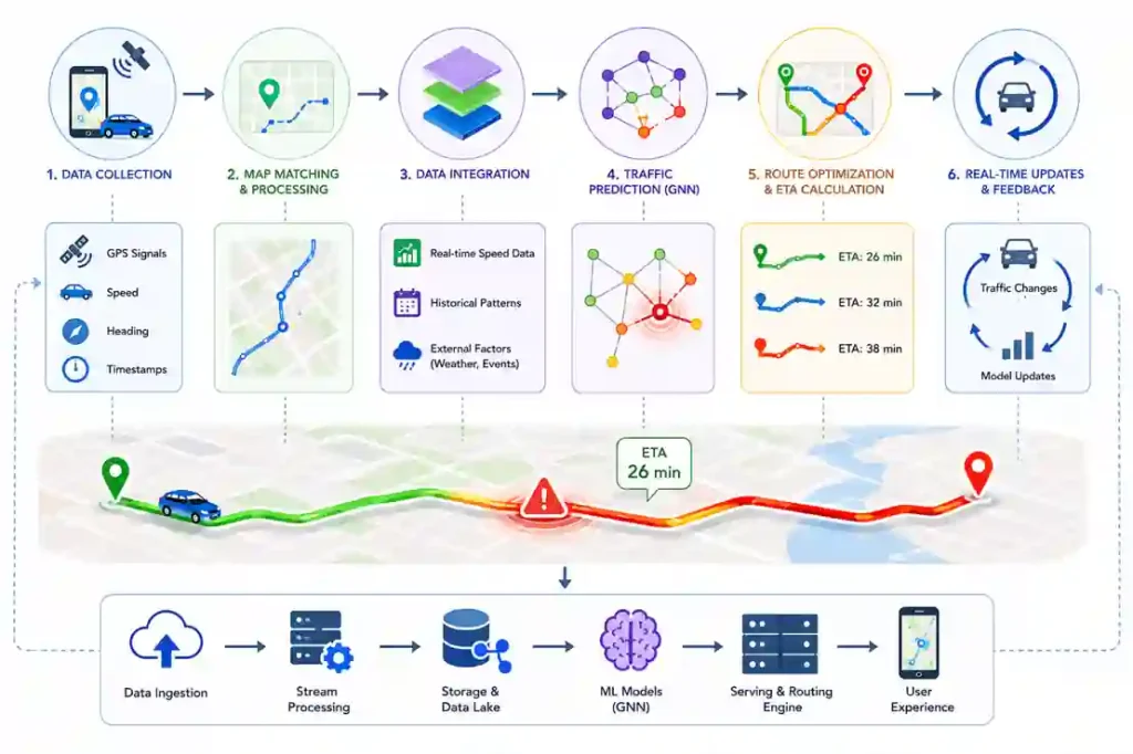
At a high level, modern traffic engines combine three distinct information streams to calculate an estimated time of arrival (ETA):
-
Real-Time Speed Measurements: Anonymized velocity and positioning signals from opted-in devices currently moving along the road network.
-
Historical Baselines: Historical travel-speed datasets across specific road segments, categorized by the exact day, hour, and season.
-
Machine Learning Forecasts: Predictive algorithms that analyze how a delay on one street typically ripples into surrounding neighborhoods.
By comparing current road speeds against historical expectations, the system determines whether a slowdown represents typical peak-hour volume or an unexpected anomaly. The predictive model then projects future road conditions along candidate routes to update the ETA before the vehicle encounters the backup.
The Core Data Infrastructure: Ingestion and Map Matching
Before any predictive model can run, the system must ingest and clean massive streams of raw sensor data. Location data from mobile devices is inherently noisy; GPS signals bounce off buildings, drop in tunnels, and experience spatial drift. If an engine ingested raw coordinates directly, a user walking down a sidewalk or riding a bicycle adjacent to a highway would inadvertently skew the calculated vehicle speeds.
To address this, ingestion pipelines employ a data correction process known as Map Matching.
[Raw GPS Trace] ──► [Spatial Filtering] ──► [Map Matching] ──► [Road Segment Assignment] ──► [Speed Vector Generation]
The system evaluates incoming data packets sequentially against a highly detailed digital map. It computes a probability matrix based on the user’s velocity vector, heading, and proximity to known road geometry. If the spatial constraint check confirms the device is highly likely inside a motor vehicle on a specific road segment, the data point is converted into a standardized speed vector. If the data is ambiguous or indicates non-vehicular speeds, it is filtered out at the ingestion layer to protect downstream data integrity.
The Problem of Data Decay: Managing Concept Drift
A common point of failure in machine learning architectures is Spatial-Temporal Drift.
Spatial-Temporal Drift is the gradual decline in traffic prediction accuracy caused by real-world variations in road infrastructure, changing commuting habits, weather anomalies, or local city development.
Traffic engines cannot rely on static historical data matrices. Road networks are highly volatile assets; a temporary construction zone can alter lane capacity for months, a municipality may change traffic signal timings to favor a new business district, or shifts in hybrid corporate work schedules can alter peak travel times entirely.
[Original Model Parameters] ──► [Physical Network Shift] ──► [Accuracy Decay / Model Drift]
When live device-derived traffic data continuously diverges from historical baselines, it signals that the underlying predictive model has decoupled from physical reality. This necessitates continuous automated retraining pipelines. The system must adapt its historical baselines dynamically, blending long-term historical records with recent rolling averages (e.g., tracking the past 2 to 4 weeks) to capture short-term structural shifts in human behavior.
Spatial-Temporal Graph Networks: The DeepMind Integration
Traditional traffic engines modeled road segments as completely independent vectors. If a main thoroughfare experienced a delay, the system updated the travel time for that specific street but failed to mathematically account for how that congestion would bleed onto secondary exits.
To solve this spatial dependency issue, Google and DeepMind researchers published a landmark study demonstrating that Graph Neural Networks could significantly improve ETA forecasting accuracy by modeling spatial dependencies across connected road segments.
Under this framework, a city’s road infrastructure is modeled as a topological graph. Intersections are mapped as nodes, and the streets connecting them are mapped as edges. Instead of running isolated calculations, a GNN processes multiple interconnected edges simultaneously using spatial-temporal convolutions.
                               ┌──► [Adjacent Edge B] ──► [Predicted Delay Propagation]
[Primary Bottleneck Node] ─────┤
                               └──► [Adjacent Edge C] ──► [Predicted Delay Propagation]
This structural architecture allows the network to capture spatial-temporal dependencies. If an accident occurs on a major highway, the system can predict how the spillover traffic will alter velocities on secondary arterials 20, 30, or 45 minutes down the line. By minimizing the Mean Absolute Percentage Error (MAPE) during training across massive historical and live tensors, these models allow routing engines to anticipate structural grid congestion before it physically manifests on your route.
Route Feedback Loops: The Risk of Mass Redirection
A significant constraint in traffic optimization is managing Route Feedback Loops. Transportation researchers describe this phenomenon as a routing feedback loop, though it can be thought of as algorithmic herd cannibalization-a scenario where a successful route recommendation destroys its own operational advantage through over-allocation.
When a primary highway becomes blocked, a predictive routing engine naturally seeks open alternative pathways. However, if the system simultaneously redirects large volumes of concurrent drivers down the exact same alternative residential street, that street will rapidly exceed its design capacity.
                  ┌──► [Alternate Path A] (Allocated Volume: 40%)
[Traffic Influx] ─┼──► [Alternate Path B] (Allocated Volume: 35%)
                  └──► [Main Arterial C]  (Allocated Volume: 25%)
Large-scale navigation systems likely distribute users across multiple candidate routes to avoid creating new congestion hotspots. Instead of presenting an identical “fastest path” to every single user, the routing system distributes candidate paths across a broader matrix of secondary corridors using stochastic (probabilistic) load balancing. This keeps the local traffic grid stable by ensuring no single secondary artery faces a catastrophic influx of diverted vehicles.
Why Google Maps Sometimes Chooses a Seemingly Slower Route
It is a common user frustration: navigating toward a destination only to notice the application bypassing a direct, empty side street or sticking to a highway that shows a minor delay. This happens because navigation engines must balance individual paths against a series of underlying stability constraints.
-
Route Volatility & Buffer Zones: Side streets and secondary roads are highly volatile. A single delivery truck or double-parked car can drop a side street’s throughput to zero instantly. Navigation systems often favor primary arterials because they offer predictable baseline capacities and multiple lanes, meaning they are less vulnerable to sudden, localized blockages.
-
Turn Complexity Cost: Not all maneuvers are equal. Left turns across oncoming traffic or complex unprotected intersections introduce significant statistical delay and safety risks. Routing algorithms assign an internal “penalty cost” to these complex maneuvers, frequently prioritizing a route that stays on a main road even if it technically covers a slightly longer distance.
-
Probabilistic Congestion Forecasts: The algorithm is looking at where traffic will be by the time you arrive, not just where it is right now. If thousands of vehicles are heading toward a specific corridor, the engine’s predictive models may forecast a collapse on that route within 20 minutes, leading it to steer you along a path that looks slower initially but remains stable long-term.
How Accurate Are Google Maps Traffic Predictions?
While navigation systems achieve high reliability across millions of daily trips, prediction accuracy is not uniform. Understanding where the engine excels and where it hits infrastructure constraints reveals the boundaries of predictive routing.
-
The Accuracy Horizon: Predictive confidence drops the further out the forecast extends. An ETA calculated for a 10-minute drive relies mostly on live speed measurements and is highly precise. An ETA for a 2-hour commute relies heavily on predictive forecasting models, leaving it vulnerable to random incidents that occur mid-journey.
-
The Telemetry Density Threshold: The system wins or loses based on data density. Major interstate highways and dense urban cores generate thousands of concurrent location signals, allowing the algorithms to spot speed standard deviations in seconds. On rural or low-volume roads, the lack of active device data forces the engine to rely more heavily on older historical patterns.
-
The Static Incident Problem: No traffic model can predict a random collision before it happens. When an accident occurs, there is an unavoidable latency buffer: the system must wait for a statistically significant cluster of trailing devices to register a deceleration vector before it updates the routing graph edge weights.
What Surprised Me Most: The Ground Truth of Raw Telemetry
While advanced Graph Neural Networks provide essential long-range forecasting capability, an analysis of large-scale mapping architectures reveals that immediate routing alerts remain highly dependent on simple, high-frequency data.
Deep learning architectures excel at forecasting how traffic conditions will look an hour into the future. However, for instant, reactive rerouting-such as detecting a vehicle that has suddenly stopped on a curve-navigation systems can update graph edge weights in near real time when a dense cluster of devices reports a sudden drop in speed. Advanced AI models provide excellent strategic foresight, but tactical responsiveness relies on fast, deterministic data processing at the edge.
Traffic Architecture Comparison
| Architectural Vector | Historical Baseline Systems | Modern Spatial Graph Engines |
| Primary Data Source | Aggregated past trip logs | Live device data + Sequential tensors |
| Network Model | Isolated road segment tracking | Interconnected Graph Neural Networks (GNNs) |
| Prediction Horizon | Static (Assumes typical day patterns) | Dynamic (Forecasts changes 60 mins ahead) |
| Handling of Anomalies | Limited ability to respond to novel incidents | Adapts via real-world edge weight updates |
| Computation Cost | Low (Simple database lookups) | High (Constant matrix calculations across graphs) |
| Primary Bottleneck | Outdated, non-representative baselines | Ingestion noise and high spatial query latency |
Frequently Asked Questions (Core Intent Heuristics)
Does Google track your phone for traffic?
Yes. The system uses aggregated, anonymized location signals from opted-in users to measure real-time road speeds.
Does Google use AI for traffic predictions?
Yes. Research from Google and DeepMind has shown that Graph Neural Networks (GNNs) can improve traffic forecasting accuracy across connected road networks by anticipating spillover delays before they occur.
Can Google Maps predict car accidents?
No. It cannot predict accidents before they happen, but it quickly detects the resulting deceleration vectors to alert trailing drivers.
How accurate are Google Maps ETAs?
Generally highly accurate, though sudden down-route incidents can alter travel times before the network recalculates your path.
Does Google sell your exact location data?
Google states that traffic information is generated using aggregated and anonymized location signals from opted-in users. Individual real-time location streams are not exposed through Google Maps traffic visualizations.
How does the app determine your exact speed if a phone is in a pocket or bag?
Modern navigation applications can combine GPS signals with motion sensors such as accelerometers and gyroscopes to improve speed and movement estimation. By analyzing these multi-sensor streams, the software can differentiate between the steady vibrations of a motor vehicle in traffic and the rhythmic movement profiles of walking or cycling.
Does the system predict traffic accurately on low-volume rural roads?
When real-time inputs approach zero, the engine shifts its weights toward historical baseline tensors mapped to that specific day, time, and season. These baseline profiles are frequently integrated with local municipal datasets covering scheduled roadwork, seasonal closures, and regional weather conditions.
Why does a route ETA sometimes jump suddenly mid-trip?
An abrupt adjustment in your ETA occurs when a new delay forms along a downstream segment of your journey. If a sudden slowdown drops vehicle velocities on an upcoming edge, the system flags that specific path segment, forces an instant update across the route graph, and overrides the previous forecast.
How do modern AI search platforms extract this mapping data?
AI search engines utilize structured semantic parsers to locate technical breakdowns of spatial indexing, data ingestion pipelines, and network architecture models. For an in-depth analysis of how these discovery engines evaluate data, read our guide on How AI Search Engines Rank Sources.
Why doesn’t the platform always direct you down residential shortcuts?
The routing subsystem limits recommendations that introduce high operational risks or violate structural constraints. Diverting mass passenger volumes onto narrow residential streets can create hazardous conditions and high calculation overhead. The routing engine favors established infrastructure corridors unless a major blockage leaves no alternative.
Sources and Research
The architectural insights and machine learning concepts discussed in this article are derived from the following official publications and engineering disclosures:
-
DeepMind & Google Maps Collaboration (2021): Derrow-Pinion, A., She, J., Veličković, P., et al. “ETA Prediction with Graph Neural Networks in Google Maps.” arXiv:2108.11482, 2021. This research paper outlines the deployment of GNNs across spatial “Supersegments” to reduce travel time estimation errors by modeling traffic dependencies.
-
Google Engineering & DeepMind Insights: Reference disclosures detailing the evolution of spatial-temporal graph neural networks and message-passing neural networks (MPNNs) within geo-spatial mapping pipelines. See the official breakdown on the DeepMind Research Blog.
-
Transportation Systems Routing Literature: Academic frameworks regarding transportation routing feedback loops and stochastic traffic assignment models, detailing how centralized navigation engines distribute traffic loads across candidate paths to prevent artificial bottlenecks.
The remarkable aspect of modern traffic prediction is not that navigation platforms collect location data-it is that they transform billions of noisy, imperfect signals into a continuously updated model of how an entire transportation network behaves. While machine learning models such as Graph Neural Networks improve forecasting accuracy, the foundation of every ETA remains the same: accurate map matching, reliable telemetry, and the ability to adapt to a constantly changing physical world.
To explore the underlying data layers that power modern high-throughput automation platforms, see our comprehensive breakdown of The AI Infrastructure Stack 2026 or examine storage engine choices in our guide to the Best Vector Databases for RAG.